Snowflake's huge popularity is driven by its ability to process large volumes of data at extremely low latency with minimal configuration. As a result, it is an established favorite of data teams across thousands of organizations. In this guide, we share optimization techniques to maximize the performance and efficiency of Snowflake. Follow these best practices to make queries run faster while also reducing costs.

All the Snowflake performance tuning techniques discussed in this post are based on the real world strategies SELECT has helped over 100 Snowflake customers employ. If you think there's something we've missed, we'd love to hear from you! Reach out via email or use the chat bubble at the bottom of the screen.

Snowflake Query Optimization Techniques

The Snowflake query performance optimization techniques in this post broadly fall into three separate categories:

1. Improve data read efficiency

Queries can sometimes spend considerable time reading data from table storage. This step of the query is shown as a TableScan in the query profile. A TableScan involves downloading data over the network from the table's storage location into the virtual warehouse's worker nodes. This process can be sped up by reducing the volume of data downloaded, or increasing the virtual warehouse's size.

Snowflake only reads the columns which are selected in a query, and the micro-partitions relevant to a query's filters - provided that the table's micro-partitions are well-clustered on the filter condition.

The four techniques to reduce the data downloaded by a query and therefore speed up TableScans are:

• Reduce the number of columns accessed
• Leverage query pruning & table clustering
• Use clustered columns in join predicates
• Use pre-aggregated tables

2. Improve data processing efficiency

Operations like Joins, Sorts, Aggregates occur downstream of TableScans and can often become the bottleneck in queries. Strategies to optimize data processing include reducing the number of query steps, incrementally processing data, and using your knowledge of the data to improve performance.

Techniques to improve data processing efficiency include:

• Simplify and reduce the number of query operations
• Reduce the volume of data being processed by filtering early
• Avoid repeated references to CTEs
• Remove un-necessary sorts
• Prefer window functions over self-joins
• Avoid joins with an OR condition
• Use your knowledge of the data to help Snowflake process it efficiently
• Avoid querying complex views
• Ensure effective use of the query caches

3. Optimize warehouse configuration

Snowflake's virtual warehouses can be easily configured to support larger and higher concurrency workloads. Key configurations which improve performance are:

• Increase the warehouse size
• Increase the warehouse cluster count
• Change the warehouse scaling policy

Before diving into optimizations, let's first remind ourselves how to identify what's slowing a query down.

How to optimize a Snowflake Query

Before you can optimize a Snowflake query, it's important to understand what the actual bottleneck in the query is by leveraging query profiling. Which operations are slowing it down, and where should you consequently focus your efforts?

To figure this out, use the Snowflake Query Profile (query plan), and look to the 'Most Expensive Nodes' section. This tells you which parts of the query are taking up the most query execution time.

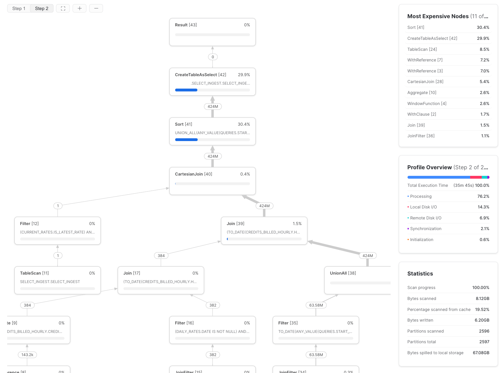
In this example, we can see the bottleneck is the Sort step, which would indicate that we should focus on improving the data processing efficiency, and possibly increase the warehouse size. If a query's most expensive node(s) are TableScans, efforts will be best spent optimizing the data read efficiency of the query.

1. Select fewer columns

This is a simple one, but where it's possible, it makes a big difference. Query requirements can change over time, and columns that were once useful may no longer be needed or used by downstream processes. Snowflake stores data in a hybrid-columnar file format called micro-partitions. This format enables Snowflake to reduce the amount of data that has to be read from storage. The process of downloading micro-partition data is called scanning, and reducing the number of columns results in less data transfer over the network.

2. Leverage query pruning

To reduce the number of micro-partitions scanned by a query, a technique known as query pruning, a few things need to happen:

1. Your query needs to include a filter which limits the data required by the query. This can be an explicit where filter or an implicit join filter.
2. Your table needs to be well clustered on the column used for filtering.

Running the below query against the hypothetical orders table shown in the diagram will result in query pruning since (a) the orders table is clustered by created_at (the data is sorted by created_at) and (b) the where clause explicitly filters the created_at with a specific date.

select *
from orders
where created_at > '2022/08/14'

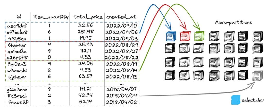
To determine whether pruning performance can be improved, take a look at the query profile's Partitions scanned and Partitions total statistics.

If you're not using a where clause filtering in a query, adding one may speed up the TableScan significantly (and downstream nodes too as they process less data). If your query already has where clause filtering but the 'Partitions scanned' are close to the 'Partitions total', this means that the where clause is not being effectively pruned on.

Improve pruning by:

1. Ensuring where clauses are placed as early in queries as possible, otherwise they may not be 'pushed down' onto the TableScan step (this also speeds up later steps in the query)
2. Adding well-clustered columns to join and merge conditions which can be pushed down as JoinFilters to enabling pruning
3. Making sure that columns used in where filters of a query align with the table's clustering (learn more about clustering here)
4. Avoiding the use of functions in where conditions - these often prevent Snowflake from pruning micro-partitions

3. Use clustered columns in join predicates

The most common form of pruning most users will be familiar with is static query pruning. Here’s a simple example, similar to the one above:

select *
from orders
where order_date > current_date - 7

If the orders table is clustered by order_date, Snowflake’s query optimizer will recognize that most micro-partitions (files) containing data older than 7 days ago can be ignored. Since scanning remote data will requires significant processing time, eliminating micro-partitions will greatly increase the query speed.

A lesser known feature of Snowflake’s query engine is dynamic pruning. Compared to static pruning which happens before execution during the query planning phase, dynamic query pruning happens on the fly as the query is being executed.

Consider a process that regularly updates existing records in the orders table through a MERGE command. Under the hood, a MERGE requires a join between the source table containing the new/updated records and the target table (orders) that we want to update.

Dynamic pruning kicks in during the join. How does it work? As the Snowflake query engine reads the data from the source table, it can identify the range of records present and automatically push down a filter operation to the target table to avoid un-necessary data scanning.

Let’s ground this in an example. Imagine we have a source table containing 3 records we need to update in the target orders table, which is clustered by order date. A typically MERGE operation would match records between the two tables using a unique key, such as order key. Because these unique keys are usually random, they won’t force any query pruning. If we instead modify the MERGE condition to match records on both order key and order date, then dynamic query pruning can kick in. As Snowflake reads data from the source table, it can detect the range of dates covered by the 3 orders we are updating. It can then push down that range of dates into a filter on the target side to prevent having to scan that entire large table.

How can you apply this to your day to day? If you currently have any MERGE or JOIN operations where significant time is spent scanning the target table (on the right), then consider whether you can introduce additional predicates to your join clause that will force query pruning. Note, this will only work if (a) your target table is clustered by some key (b) the source table (on the left) you are joining to contains a tightly bound range of records on the cluster key (i.e. a subset of order dates).

{{ config(
    materialized='incremental',
    unique_key=['order_id', 'updated_at'],
) }}

select *
from {{ ref('stg_orders') }}
...

4. Use pre-aggregated tables

Create 'rollup' or 'derived' tables that contain fewer rows of data. Pre-aggregated tables can often be designed to provide the information most queries require while using less storage space. This makes them much faster to query. For retail businesses, a common strategy is to use a daily orders rollup table for financial and stock reporting, with the raw orders table only queried where per-order granularity is needed.

5. Simplify!

Each operation in a query takes time to move data around between worker threads. Consolidating and removing unnecessary operations reduces the amount of network transfer required to execute a query. It also helps Snowflake reuse computations and save additional work. Most of the time, CTEs and subqueries do not impact performance, so use them to help with readability.

In general, having each query do less makes them easier to debug. Additionally, it reduces the chance of the Snowflake query optimizer making the wrong decision (i.e. picking the wrong join order).

6. Reduce the volume of data processed

The less data there is, the faster each data processing step completes. Reducing both the number of columns and rows processed by each step in a query will improve performance.

Here's an example where moving a qualify filter earlier in the query resulted in a 3X increase in query runtime. The first query profile shows the runtime when the QUALIFY filter happened after a join.

Because the QUALIFY filter didn't require information after the join, it could be moved earlier in the query. This results in significantly less data being joined, vastly improving performance:

For transformation queries that write to another table, a powerful way of reducing the volume of data processed is incrementalization. For the example of the orders table, we could configure the query to only process new or updated orders, and merge those results into the existing table.

7. Repeating CTEs can be faster, sometimes

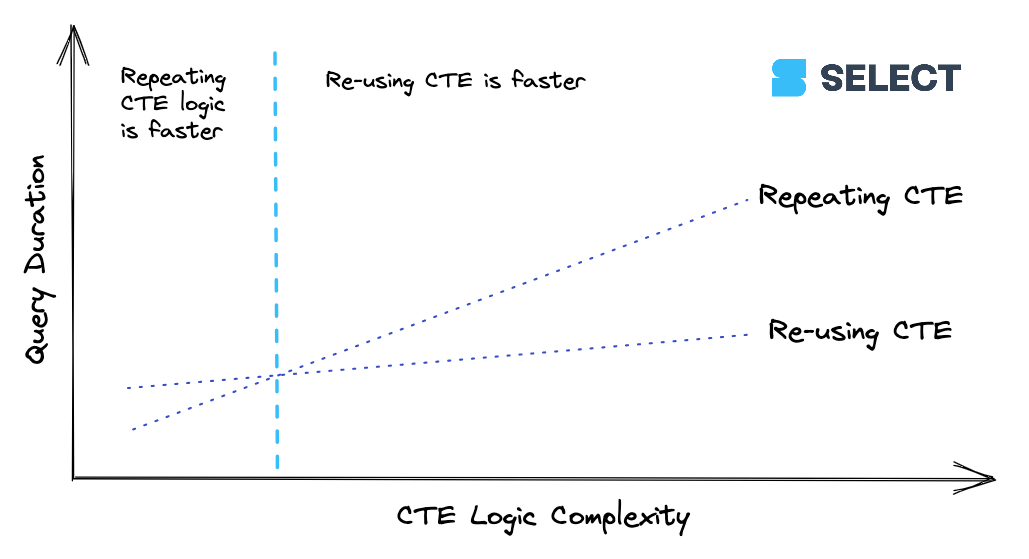
We've previously written about whether you should use CTEs in Snowflake. Whenever you reference a CTE more than once in your query, you will see a WithClause operation in the query profile (see example below). In certain scenarios, this can actually make the query slower and it can be more efficient to re-write the CTE each time you need to reference it.

When a CTE reaches a certain level of complexity, it’s going to be cheaper to calculate the CTE once and then pass its results along to downstream references rather than re-compute it multiple times. This behavior isn’t consistent though, so it’s best to experiment. Here’s a way to visualize the relationship:

8. Remove un-necessary sorts

Sorting is an expensive operation, so be sure to remove any sorts that are not required:

9. Prefer window functions over self-joins

Rather than using a self join, try and use window functions wherever possible, as self joins are very expensive since they result in a join explosion:

10. Avoid joins with an OR condition

Similar to self-joins, joins with an OR join condition result in a join explosion since they are executed as a cartesian join with a post filter operation. Use two left joins instead:

11. Use your knowledge of the data to help Snowflake process it efficiently

Your own knowledge of the data can be used to improve query performance. For example, if a query groups on many columns and you know that some of the columns are redundant as the others already represent the same or a higher granularity, it may be faster to remove those columns from the group by and join them back in in a separate step.

If a grouped or joined column is heavily skewed (meaning a small number of distinct values occur most frequently), this can have a detrimental impact on Snowflake's speed. A common example is grouping by a column that contains a significant number of null values. Filtering rows with these values out and processing them in a separate operation can result in faster query speeds.

Finally, range joins can be slow in all data warehouses including Snowflake. Your knowledge of the interval lengths in the data can be used to reduce the join explosion that occurs. Check out our recent post on this if you're seeing slow range join performance.

12. Avoid complex views

As a best practice, avoid creating and using any complex views in your queries. Views should be used to persist simple data transformations like renaming columns, basic column calculations, or for data models with lightweight joins.

To understand how complex views can wreak havoc, consider the following, seemingly innocent query:

select
    a.*,
    b.*
from model_a as a
left join model_b as b
    on a.id=b.id

This query was repeatedly taking >45 minutes to run, and failing due to a "Incident".

When digging into the query profile (also referred to as the "query plan"), you can see that the models being queried were actually complex views, with hundreds of tables.

The solution here is to split up the complex view into simpler, smaller parts, and persist them as tables.

13. Ensure effective use of the query caches

Each node in a virtual warehouse contains local disk storage which can be used for caching micro-partitions read from remote storage. If multiple queries access the same set of data in a table, the queries can scan the data from the local disk cache instead of remote storage, which can speed up a query if the primary bottleneck is reading data.

When the warehouse suspends, Snowflake doesn't guarantee that the cache will persist when the warehouse is resumed. The impact of cache loss is that queries have to re-scan data from table storage, rather than reading it from the much faster local cache. If warehouse cache loss is impacting queries, increasing the auto-suspend threshold will help.

Separately, Snowflake has a global result cache which will return results for identical queries executed within 24 hours provided that data in the queried tables is the same. There are certain situations which can prevent the global result cache from being leveraged (i.e. if your query has a non-deterministic function), so be sure to check that you are hitting the global result cache when expected. If not, you may need to tweak your query or reach out to support to file a bug.

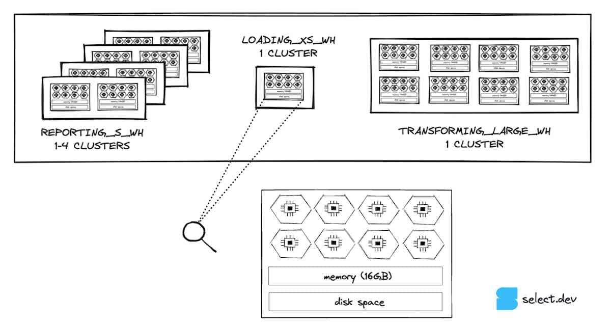
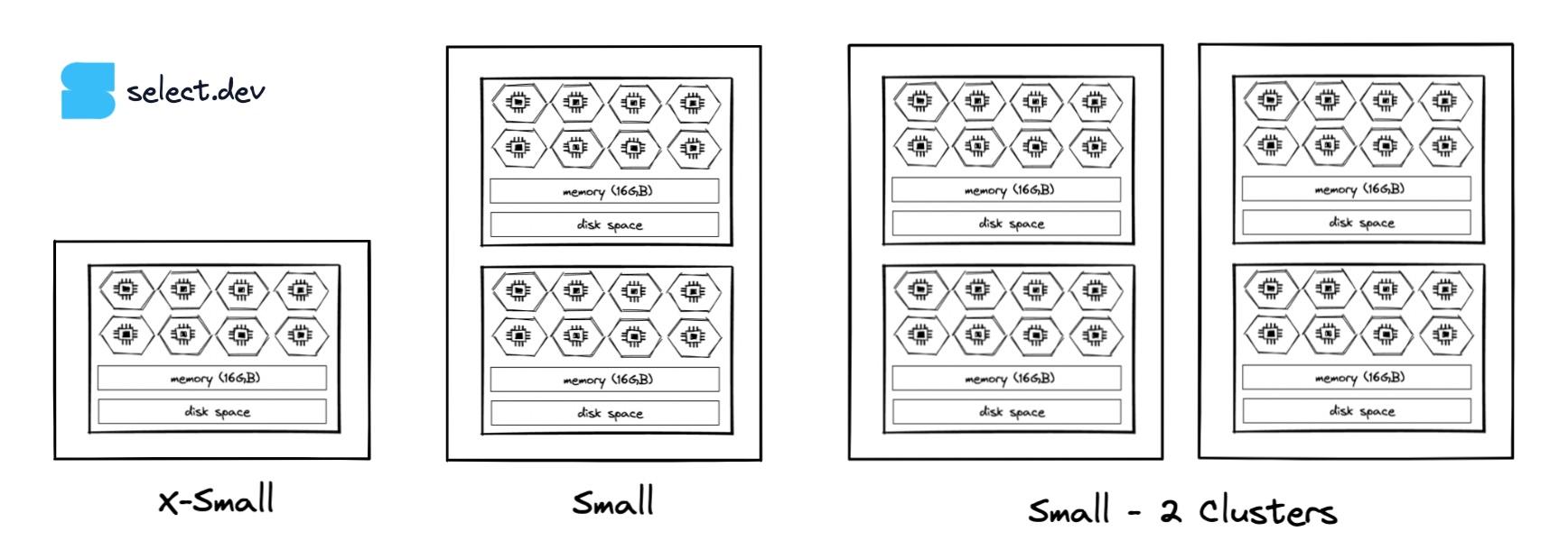
14. Increase the warehouse size

Warehouse size determines the total computational power available to queries running on the warehouse, also known as vertical scaling.

Increase virtual warehouse size when:

1. Queries are spilling to remote disk (identifiable via the query profile)
2. Query results are needed faster (typically for user-facing applications)

Queries that spill to remote disk run inefficiently due to the large volumes of network traffic between the warehouse executing the query, and the remote disk that store data used in executing the query. Increasing the warehouse size doubles both the available RAM and local disk, which are significantly faster to access than remote disk. Where remote disk spillage occurs, increasing the warehouse size can more than double a query's speed. We've gone into more detail on Snowflake warehouse sizing in the past, and covered how to configure warehouse sizes in dbt too.

Note, if most of the queries running on the warehouse don't require a larger warehouse, and you want to avoid increasing the warehouse size for all queries, you can instead consider using Snowflake's Query Acceleration Service. This service, available on Enterprise edition and above, can be used to give queries that scan a lot of data additional compute resources.

15. Increase the Max Cluster Count

Multi-cluster warehouses, available on Enterprise edition and above, can be used to create more instances of the same size warehouse.

If there are periods where warehouse queuing causes queries to not meet their required processing speeds, consider using multi-clustering or increasing the maximum cluster count in a warehouse. This will allow the warehouse to track query volumes by adding or removing clusters.

Unlike warehouse cluster count, Snowflake cannot automatically adjust the size of virtual warehouses with query volumes. This makes multi-cluster warehouses more cost-effective for processing volatile query volumes, as each cluster is only billable while in an active state.

16. Adjust the Cluster Scaling Policy

Snowflake offers two scaling policies - Standard and Economy. For all virtual warehouses which serve user-facing queries, use the Standard scaling policy. If you're very cost-conscious, experiment with the Economy scaling policy for queueing-tolerant workloads such as data loading to see if it reduces cost while maintaining the required throughput. Otherwise, we recommend using Standard for all warehouses.

Other Resources

If you are looking for more content on Snowflake query optimization, we recommend exploring the additional video resources below.

Behind the Cape: 3 Part Series on Snowflake Cost Optimization (2023)

In this 3 part video series, Ian joined Snowflake data superhero Keith Belanger for Behind the Cape, a series of videos where Snowflake experts dive into various topics.

Part 1

For this episode, we tackled the meaty topic of Snowflake cost optimization. Given we only had 30 minutes, it ended up being a higher level conversation around how to get started, Snowflake's billing model, and tools Snowflake provides to control costs.

Here is a full list of topics we discussed:

1. How should you get started with Snowflake cost optimization? (TL,DR: build up a holistic understanding of your cost drivers before diving into any optimization efforts)
2. Where most customers are today with their understanding of Snowflake usage
3. How does Snowflake's billing model work (did you know it's actually cheaper to store data in Snowflake?)
4. The tools offered by Snowflake for cost visibility
5. Methods you have to control costs (resource monitors, query timeouts, and ACCESS CONTROL - the one no one thinks of!)
6. Where should you start with cost cutting? Start optimizing queries? Or go higher level?
7. Resources for learning more.

For those looking to get an overview of cost optimization, monitoring and control, this is a great place to start. The video recording can be found below. There is so much to discuss on this topic and we didn't get to go super deep, so will have to do a follow up soon!

Part 2

In this episode we go deeper into some important foundational concepts around Snowflake query optimization:

1. The lifecycle of a Snowflake query
2. Snowflake virtual warehouse sizing
3. How to use the Snowflake query profile and identify bottlenecks

Part 3

In the final episode of the series, we dive into the most important query optimization techniques:

1. Understanding Snowflake micro-partitions
2. How to leverage query pruning
3. How to ensure your tables are effectively clustered

Snowflake Optimization Power Hour Video (2022)

On September 28, 2022, Ian gave a presentation to the Snowflake Toronto User Group on Snowflake performance tuning and cost optimization. The following content was covered:

1. Snowflake architecture
2. The lifecycle of a Snowflake query
3. Snowflake's billing model
4. A simple framework for cost optimization, along with a detailed methodology for how to calculate cost per query
5. Warehouse configuration best practices
6. Table clustering tips

Slides

The slides can be viewed here. To navigate the slides, you can click the arrows on the bottom right, or use the arrow keys on your keyboard. Press either the "esc" or the "o" key to zoom out into an "overview" mode where you can see all slides. From there, you can again navigate using the arrows and either click a slide or press "esc"/"o" to focus on it.

Presentation Recording

A recording of the presentation is available on youtube. The presentation starts at 3:29.

If you would like, I am more than happy to come in and give this presentation (or a variation of it) to your team where they can have the opportunity to ask questions. Send an email to [email protected] if you would like to set that up.

Query Optimization at Snowflake (2020)

If you'd like to better understand the Snowflake query optimizer internals, I'd highly recommend watching this talk from Jiaqi Yan, one of Snowflake's most senior database engineers: