The MERGE statement is a powerful multi-purpose tool that allows users to upsert and delete rows all at once. Instead of managing data loading pipelines through interrelated yet separate statements, MERGE enables you to significantly simplify and control them through a single atomic statement. In this post, we guide you through the features and architectural foundations of MERGE in Snowflake and discuss how to improve MERGE query performance.

What is MERGE in Snowflake?

The MERGE feature has been with us for a long time, even before the era of columnar databases was in full bloom. Also known as upsert (insert and update), it helps us handle changes properly, ensuring the consistency of data pipelines. Modern ETL jobs tend to manage endless streams of data incrementally, so MERGE can't be overlooked. It covers almost all use cases, allowing us to perform delete, insert, and update operations in a single transaction. Multiple scripts modifying the same table in parallel will longer be a headache.

Unlike an UPDATE statement, MERGE can process multiple matching conditions one after the other to complete updates or deletes. However, for unmatched records, a user is only able to insert a chunk of data from the source to the target destination. Currently, unlike in Databricks ¹ and Google BigQuery ², Snowflake doesn't allow you to specify behaviour when partial conditions are met, specifically for unmatched rows in the source table.

Let’s delve into the syntax. To use the MERGE command, you must pass the following arguments in:

1. Source table: The table containing the data to be merged.
2. Target table: The destination table where data should be synchronised.
3. Join expression: The key fields from both tables link tables together
4. Matched clause: At least one (non-)matched clauses determining your expected outcome

Using MERGE to update customer active status

Let’s start by looking at an example of a customer table which we would like to update from a source table containing new customer data. We'll use customer_id to match the records in each table. To demonstrate how the MERGE handles both updates and inserts, the generated table data is partially overlapped.

-- Creating Tables
CREATE OR REPLACE TABLE target_table (
 customer_id NUMBER,
 is_active BOOLEAN,
 updated_date DATE
)
;

CREATE OR REPLACE TABLE source_table (
 customer_id NUMBER,
 is_active BOOLEAN
)
;

-- Inserting test values
INSERT INTO target_table VALUES
(1, TRUE, '2023-01-01'),
(2, TRUE, '2023-02-01'),
(3, FALSE, '2023-03-01')
;

INSERT INTO source_table VALUES
(1, FALSE), -- update record
(2, TRUE), -- update record
(4, TRUE) -- new record
;

-- UPSERT STARTS HERE
-- Insert a missing row and update the existing ones
MERGE INTO target_table tgt
USING source_table src 
 ON tgt.customer_id = src.customer_id
WHEN MATCHED THEN
 UPDATE SET
   tgt.is_active = src.is_active,
   tgt.updated_date = '2023-04-01'::DATE
WHEN NOT MATCHED THEN
 INSERT
   (customer_id, is_active, updated_date)
 VALUES
 (src.customer_id, src.is_active, '2023-04-01'::DATE)
; 

-- Output
| Number of Rows Inserted | Number of Rows Updated |
|-------------------------|------------------------|
|           1             |           2            |

So, we’ve made an upsert resulting in updating 2 rows (ID: 1, 2) and inserting 1 new row (ID: 4). The remaining customer (ID: 3) is untouched as there are no matched rows from the source table. This simple example shows basic features of the operator and how it can be used in your project.

Let’s move forward and find out what happens under the hood.

Understanding and improving MERGE query performance

The Snowflake query profile for the "customers" MERGE query from above is shown below.

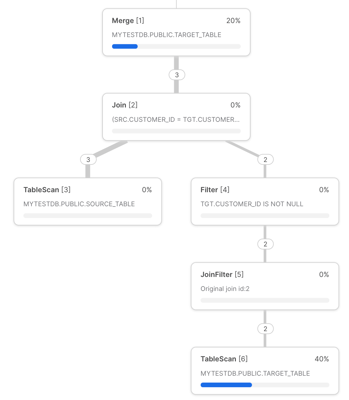
We can use this profile to illustrate potential bottlenecks:

1. Every time you run MERGE query it starts by scanning the target table. This is one of the most time consuming steps of this query. To reduce the time spent scanning data, users need to filter the target table on one of the column's it is well clustered. Doing this enables query pruning, which helps the Snowflake query execution from scanning un-needed micro-partitions. Later in the post, we'll demonstrate one way this can be achieved through dynamic pruning.
2. Right before MERGE, tables are joined via LEFT OUTER JOIN (if NON MATCHED clause is present) or INNER JOIN (for MATCHED clause only). As usual with joins, users should avoid row explosion wherever possible as they tend to lead to disk spillage due to the excessive memory requirements.
   1. One cause of poor JOIN performance can be a result of the Snowflake optimizier choosing a suboptimal join order. Users can explore manual join control option to force Snowflake to use a different join order.
   2. Take advantage of range join optimizations if the join condition involves a non-equi join.
   3. Ensure the source table has unique key fields when joined, otherwise, you will retrieve an error message unless you switch on non-deterministic behaviour.
3. In the final MERGE operation at the top of the query plan, we unfortunately can't dig deeper into the allocation time for the underlying steps taking place. The time spent on this step will be proportional to the number of volume of files and data being written.

The impact of Snowflake's architecture on MERGE

As discussed in previous a post, Snowflake's architecture involves separate storage, compute and cloud services layers. Since Snowflake's storage layer uses immutable files named micro-partitions, neither partial updates nor appends to existing files are available. Therefore, statements including insert, update, or delete trigger full overwriting ³ (or re-writing) of these files.

Whenever you make modifications to a table, two events occur simultaneously: Snowflake keeps a copy of the old data and retains it based on the Time Travel configuration ⁴, and the updated table is stored by rewriting all the necessary files.

To be more precise, a table consists of metadata pointers determining which micro-partitions are valid at any given point in time. In fact, Snowflake calls it a table version, which in turn is composed of a system timestamp, a set of micro-partitions, and partition-level statistics ⁵.

• INSERT primarily involves the addition of new micro-partitions. Beyond commonly followed strategies such as fitting warehouse size for optimal configuration and avoiding Snowflake as a high-frequency ingest platform for OLTP tasks, there is unlikely to be much room for further improvement of this step.
• UPDATEs are trickier, as a first step, it requires scanning all micro-partitions, which can become very expensive for larger tables. Ideally, updated data corresponds to a narrow date interval, so you won’t end up rewriting multiple files. Avoiding common pitfalls of joining tables, discussed earlier, are generally useful here as well.

Alternatives to MERGE

Other than MERGE, there are a couple of well-known manual options you can rely on for your data loading needs. If atomicity isn’t required and you deal with full data replacement, DELETE + INSERT is a viable strategy. Users are responsibile for finding the records that need to be deleted, and then inserting the new records in two separate statements. If the INSERT statement fails, the table will be left in a state where records are missing. Users can also execute the UPDATE and INSERT statements separately. However, since each statement must separately scan the data in the target table, this will end up consuming more compute credits.

More examples of using MERGE

Let’s continue exploring the MERGE concept with a couple of advanced examples. For these examples, we'll take advantage of the order table from the tpch_sf1000 dataset.

-- Table Size: 1.6 billion records
CREATE OR REPLACE TABLE mytestdb.public.orders AS
SELECT
  o_orderkey,
  o_custkey,
  o_orderstatus,
  o_totalprice,
  o_orderdate,
  o_orderpriority,
  o_clerk,
  o_comment,
  o_shippriority
FROM
  snowflake_sample_data.tpch_sf1000.orders
ORDER BY o_orderdate -- sorting by order
;

By adding the ORDER BY o_orderdate statement, the orders table will be well clustered by this column.

To simulate more common data loading scenarios, we delve into two examples of nearly identical MERGE statements.

MERGE, single micro-partition update values

In this first example, we will MERGE in a source dataset containing 620K records from a single day.

-- Case 1
-- Values from a single order date / micro-paritition
-- Output: ~620k rows
-- Execution time: ~17s to run

CREATE OR REPLACE TEMPORARY TABLE source_table AS
SELECT
 -- Primary Keys to Match Both Tables
 -- To cover both INSERT and UPDATE cases
 IFF(o_orderkey % 2 = 1, o_orderkey, o_orderkey + 99999999999) AS o_orderkey,
 o_orderdate,
 o_custkey,
 o_orderstatus,
 o_totalprice,
 o_orderpriority,
 o_shippriority,
 o_comment,
 -- Generate Updated Column
 UNIFORM(100000, 999999, RANDOM()) AS random_int,
 'Clerk#000' || random_int::STRING AS o_clerk -- column to update
FROM orders
WHERE o_orderdate = '1997-10-05' -- one day
;

CREATE OR REPLACE TABLE orders_q1_merge_by_key CLONE orders;

-- UPSERT
MERGE INTO orders_q1_merge_by_key target_table
USING source_table
 ON
   target_table.o_orderkey = source_table.o_orderkey
WHEN MATCHED THEN
 UPDATE SET
   target_table.o_clerk = source_table.o_clerk
WHEN NOT MATCHED THEN
 INSERT (o_orderkey, o_custkey, o_orderstatus, o_totalprice, o_orderdate, o_orderpriority, o_clerk, o_shippriority, o_comment)
 VALUES (source_table.o_orderkey, source_table.o_custkey, source_table.o_orderstatus, source_table.o_totalprice, source_table.o_orderdate, source_table.o_orderpriority, source_table.o_clerk, source_table.o_shippriority, source_table.o_comment)
;

-- Output
| Number of Rows Inserted | Number of Rows Updated |
|-------------------------|------------------------|
|           311728        |           311493       |

The query takes only 15-17 seconds to run. Half the data is updated, the other half is overwritten. This query goes through full-scan of target table, which means query pruning is inactive.

One updated row fully rewrite micro-partition

To illustrate what’s happening under the hood when we include a significant number of micro-partitions, we'll generate another source dataset with the same volume of data, about 620K rows, but this time the data will contain a range of dates in the year 1992 instead of a single day.

-- Case 2
-- Values from a single order date / micro-paritition
-- Output: ~630k rows 
-- Execution time: ~95s to run

CREATE OR REPLACE TEMPORARY TABLE source_table AS
SELECT
  -- Primary Keys to Match Both Tables
  IFF(o_orderkey % 2 = 1, o_orderkey, o_orderkey + 99999999999) AS o_orderkey
  , o_orderdate
  --  Other keys
  , o_custkey
  , o_orderstatus
  , o_totalprice
  , o_orderpriority
  , o_shippriority
  , o_comment
  -- Generate Updated Column
  , UNIFORM(100000, 999999, RANDOM()) AS random_int
  , 'Clerk#000' || random_int::STRING AS o_clerk
FROM orders SAMPLE(0.275) -- Sample 0.275% of rows in the year 1992 in order to get a similar sized source dataset
WHERE DATE_TRUNC(YEAR, o_orderdate)::DATE = '1992-01-01'
;

CREATE OR REPLACE TABLE orders_merge CLONE orders;

MERGE INTO orders_merge target_table
USING source_table
  ON
    target_table.o_orderkey = source_table.o_orderkey 
WHEN MATCHED THEN
  UPDATE SET
    target_table.o_clerk = source_table.o_clerk
WHEN NOT MATCHED THEN
  INSERT (o_orderkey, o_custkey, o_orderstatus, o_totalprice, o_orderdate, o_orderpriority, o_clerk, o_shippriority, o_comment)
  VALUES (source_table.o_orderkey, source_table.o_custkey, source_table.o_orderstatus, source_table.o_totalprice, source_table.o_orderdate, source_table.o_orderpriority, source_table.o_clerk, source_table.o_shippriority, source_table.o_comment)
;

This query takes about 95 seconds to run! Despite the same source table sizes, this query takes 4.5x longer to run!

Comparing the two MERGE examples

Let’s compare the query plan statistics to understand why the second example takes so much longer to run.

As discussed earlier, even if you only modify a single row in a table, it requires re-writing the entire micro-partition that the row belonged to. Because the source table involved data uniformly distributed across the year 1992, we have to rewrite ~6GB of data which constitutes nearly 15% of the target table size!

In many ways, this situation may be beyond your full control. If you have to update data from a full year, then you don't have many options.

Both of the examples from above involve a full scan of the target table to determine which micro-partitions need to be updated. Let's explore an optimization technique known as dynamic query pruning which can help improve the performance here.

Improving merge performance with dynamic pruning

If your MERGE query is spending a lot of time scanning the target table, then you may be able to improve the query performance by forcing query pruning which will prevent scanning un-necessary data from the target table.

Let's consider an example where we only need to update 3 different records, which take place on two different days: 1998-01-01 and 1998-02-25.

-- Source table 

CREATE OR REPLACE TEMPORARY TABLE orders_to_update AS (
SELECT
  2606029510 AS o_orderkey
  , 0 AS o_totalprice
  , DATE '1998-02-25' AS o_orderdate
UNION ALL
SELECT
  3135064003 AS o_orderkey
  , 0 AS o_totalprice
  , DATE '1998-02-25' AS o_orderdate
UNION ALL
SELECT
  5602847265 AS o_orderkey
  , 0 AS o_totalprice
  , DATE '1998-01-01' AS o_orderdate
)
;

As we saw above, a regular MERGE will just match the records on o_orderkey. Because o_orderkey is a random key, the target orders table will not be clustered by this column, and therefore the MERGE operation will have to scan the whole target table to find the micro-partitions containing the three o_orderkey values we are trying to update.

-- REGULAR MERGE

CREATE OR REPLACE TABLE orders_merge CLONE orders;

MERGE INTO orders_merge AS target
USING orders_to_update AS source
  ON
    target.o_orderkey = source.o_orderkey
WHEN MATCHED THEN
  UPDATE SET
    target.o_totalprice = source.o_totalprice
;

To eliminate having to scan all the micro-partitions in the target table, we can take advantage of the fact that the orders target table is clustered by the o_orderdate. This means that all orders with the same date will be stored in the same micro-partitions. We can modify our MERGE statement to add an additional join clause on the o_orderdate column. During query execution, Snowflake now only needs to search the micro-partitions containing orders from the dates 1998-01-01 and 1998-02-25!

This is known as dynamic pruning, because Snowflake is determining which micro-partitions to prune (avoid scanning) while during the query execution after it has read the values in the source table.

-- PRUNED MERGE

CREATE OR REPLACE TABLE orders_merge CLONE orders;

MERGE INTO orders_merge AS target
USING orders_to_update AS source
  ON
    target.o_orderkey = source.o_orderkey AND 
	  target.o_orderdate = source.o_orderdate -- PRUNING COLUMN
WHEN MATCHED THEN
  UPDATE SET
    target.o_totalprice = source.o_totalprice
;

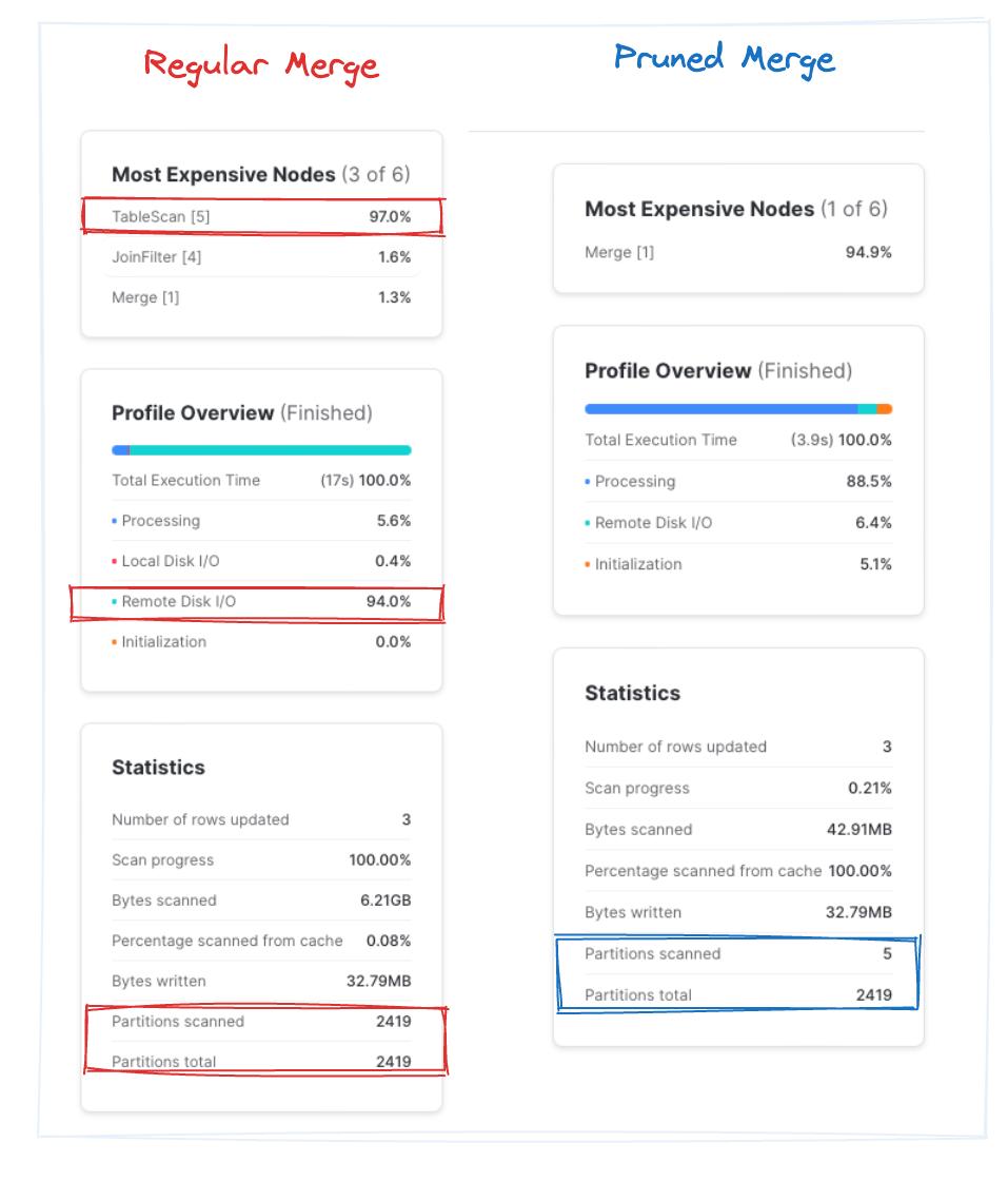
While the “regular merge” query takes ~9.5s on average across three runs, “pruned merge” finishes in ~4s. Note that in the pruned query, Snowflake quickly scanned ~0.2% of the total partitions. That’s approximately 2x improvement as a result of skipping unnecessary file blocks. Bingo!

Closing thoughts

MERGE is a great way to gracefully deal with updating and inserting data in Snowflake. By understanding Snowflake's architecture with its immutable micro-partition files, we can understand why certain MERGE operations can take a long time despite only updating a few records. We also learned how MERGE performance can be improved by minimizing the number of micro-partitions in the target table that need to be scanned.

We hope you found the post helpful, thanks for reading!

Notes

¹ Databricks delta merge into ↩

² BigQuery merge statement syntax ↩

³ The Snowflake Elastic Data Warehouse ↩

⁴ What's the Difference? Incremental Processing with Change Queries in Snowflake ↩

⁵ Zero-Copy Cloning in Snowflake and Other Database Systems ↩