The Snowflake Query Profile is the single best resource you have to understand how Snowflake is executing your query and learn how to improve it. In this post we cover important topics like how to interpret the Query Profile and the things you should look for when diagnosing poor query performance.

What is a Snowflake query plan?

Before we can talk about the Query Profile, it's important to understand what a "query plan" is. For every SQL query in Snowflake, there is a corresponding query plan produced by the query optimizer. This plan contains the set of instructions or "steps" required to process any SQL statement. It's like a data recipe. Because Snowflake automatically figures out the optimal way to execute a query, a query plan can look different than the logical order of the associated SQL statement.

In Snowflake, the query plan is a DAG that consists of operators connected by links. Operators process a set of rows. Example operations include scanning a table, filtering rows, joining data, aggregating, etc. Links pass data between operators. To ground this in an example, consider the following query:

select
  date_trunc('day', event_timestamp) as date,
  count(*) as num_events
from events
group by 1
order by 1

The corresponding query plan would look something like this:

In this plan there are 4 "operators" and 3 "links":

1. TableScan: reads the records from the events table in remote storage. It passes 1.3 million records ¹ through a link to the next operator.
2. Aggregate: performs our group by date and count operations and passes 365 records through a link to the next operator.
3. Sort: orders the data by date and passes the same 365 records to the final operator.
4. Result: returns the query results.

The Query Profile will often refer to operators as "operator nodes" or "nodes" for short. It's also common to refer to them as "stages".

What is the Snowflake Query Profile?

Query Profile is a feature in the Snowflake UI that gives you detailed insights into the execution of a query. It contains a visual representation of the query plan, with all nodes and links represented. Execution details and statistics are provided for each node as well as the overall query.

When should I use it?

The query profile should be used whenever more diagnostic information about a query is needed. A common example is to understand why a query is performing a certain way. The Query Profile can help reveal stages of the query that take significantly longer to process than others. Similarly, you can use the Query Profile to figure out why a query is still running and where it is getting stuck.

Another useful application of the Query Profile is to figure out why a query didn't return the desired result. By carefully studying the links between nodes, you can potentially identify parts of your query that are resulting in dropped rows or duplicates, which may explain your unexpected results.

How do you view a Snowflake Query Profile?

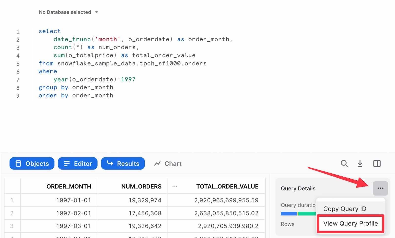
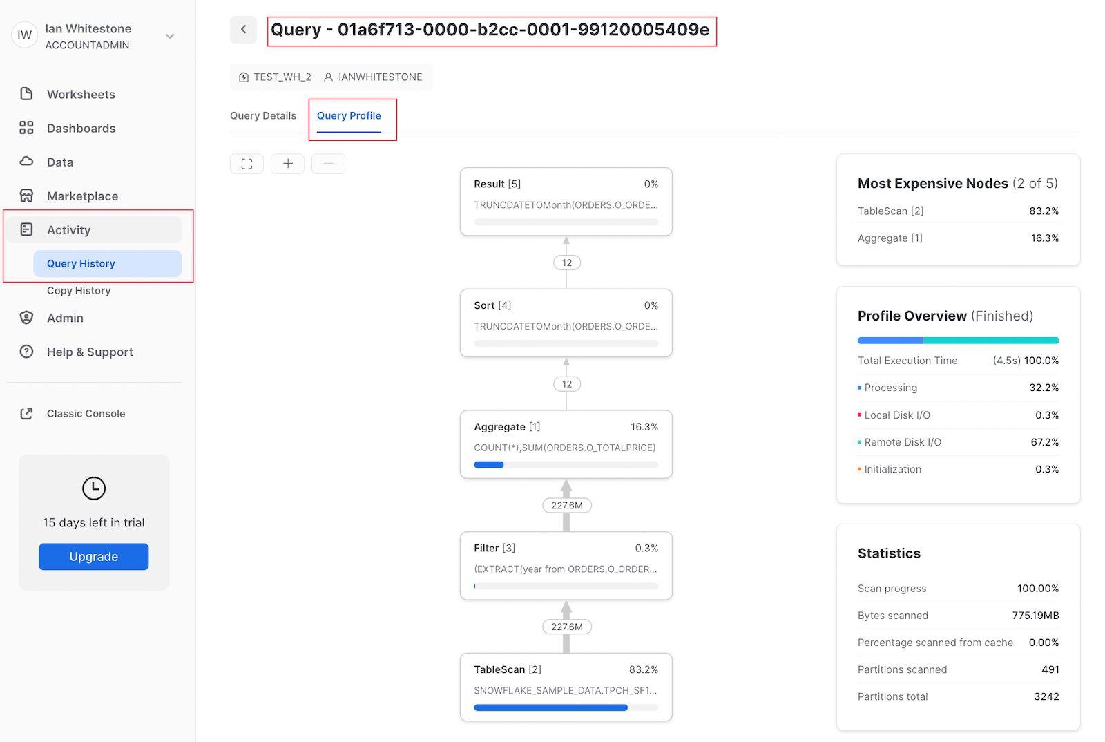
After running a query in the Snowsight query editor, the results pane will include a link to the Query Profile:

Alternatively, you can navigate to the "Query History" page under the "Activity" tab. For any query run in the last 14 days, you can click on it and see the Query Profile.

If you already have the query_id handy, you can take advantage of Snowflake's structure URLs by filling out this URL template:

• Template: https://app.snowflake.com/<snowflake-region>/<account-locator>/compute/history/queries/<paste-query-id-here>/profile
• Filled out example: https://app.snowflake.com/us-east4.gcp/xq35282/compute/history/queries/01a8c0a5-0000-0b5e-0000-2dd500044a26/profile

Can you programmatically access data in the Snowflake Query Profile?

Not yet. Snowflake is actively working on a new feature to make it possible for users to query the data shown in the Query Profile. Stay tuned.

How do you read a Snowflake Query Profile?

Basic Query

We'll start with a simple query anyone can run against the Snowflake sample dataset:

select
    date_trunc('month', o_orderdate) as order_month,
    count(*) as num_orders,
    sum(o_totalprice) as total_order_value
from snowflake_sample_data.tpch_sf1000.orders
where
    year(o_orderdate)=1997
group by order_month
order by order_month

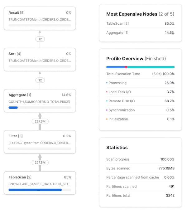
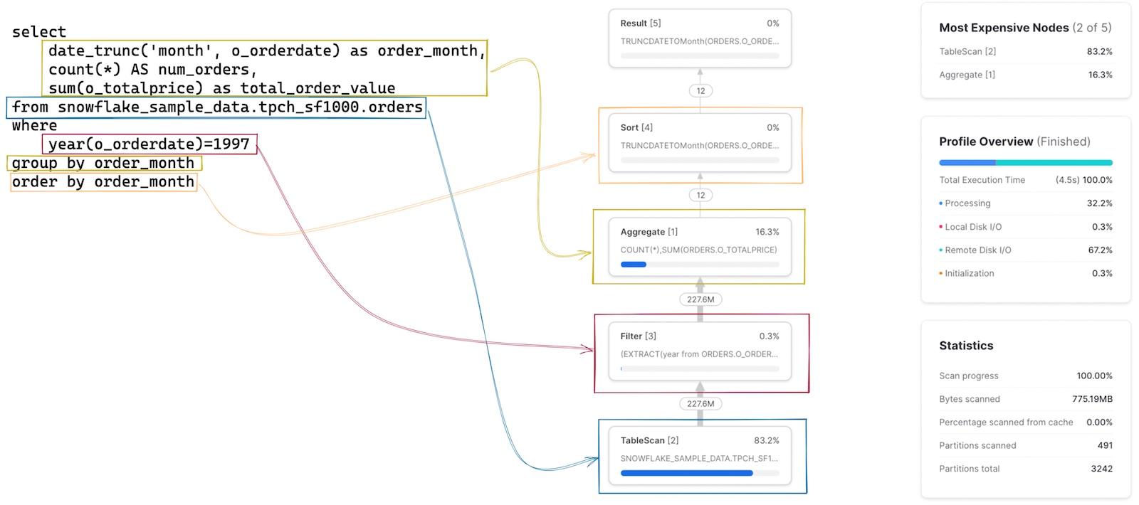
As a first step, it's important to build up a mental model of how each stage/operator in the Query Profile matches up to the query you wrote. This is tricky to do at first, but very quick once you get the hang of it. Clicking on each node will reveal more details about the operator, like the table it is scanning or the aggregations it is performing, which can help identify the relevant SQL. The SQL relevant to each operator is highlighted in the image below:

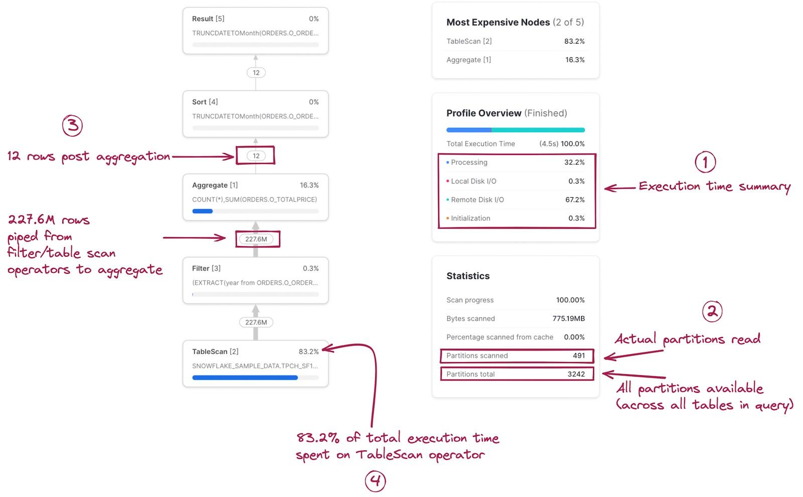
The Query Profile also contains some useful statistics. To highlight a few:

1. An execution time summary. This shows what % of the total query execution time was spent on different buckets. The 4 options listed here include:
   1. Processing: time spent on query processing operations like joins, aggregations, filters, sorts, etc.
   2. Local Disk I/O: time spent reading/writing data from/to local SSD storage. This would include things like spilling to disk, or reading cached data from local SSD.
   3. Remote Disk I/O: time spent reading/writing data from/it remote storage (i.e. S3 or Azure Blob storage). This would include things like spilling to remote disk, or reading your datasets.
   4. Initialization: this is an overhead cost to start your query on the warehouse. In our experience, it is always extremely small and relatively constant.
2. Query statistics. Information like the number of partitions scanned out of all possible partitions can be found here. Note that this is across all tables in the query. Fewer partitions scanned means the query is pruning well. If your warehouse doesn't have enough memory to process your query and is spilling to disk, this information will be reflected here.
3. Number of records shared between each node. This information is very helpful to understand the volume of data being processed, and how each node is reducing (or expanding) that number.
4. Percentage of total execution time spent on each node. Shown on the top right of each node, it indicates the percentage of total execution time spent on that operator. In this example, 83.2% of the total execution time was spent on the TableScan operator. This information is used to populate the "Most Expensive Nodes" list at the top right of the Query Profile, which simply sorts the nodes by the percentage of total execution time.

You may notice that the number of rows in/out of the Filter node are the same, implying that the year(o_orderdate)=1997 SQL code did not accomplish anything. The filter is eliminating records though, as this table contains 1.5 billion records. This is an unfortunate pitfall of the Query Profile; it does not show the exact number of records being removed by a particular filter.

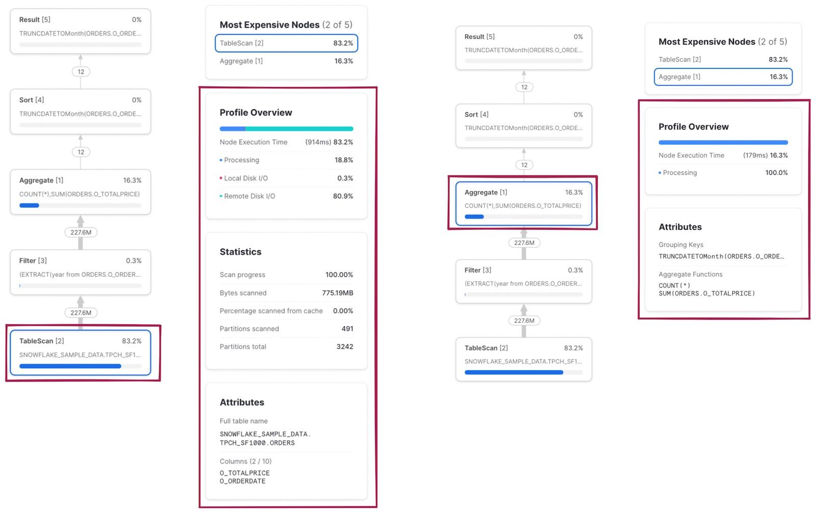
As mentioned earlier, you can click on each node to reveal additional execution details and statistics. On the left, you can see the results of clicking on the TableScan operator. On the right, the results of the Aggregate operator are shown.

Multi-step Query

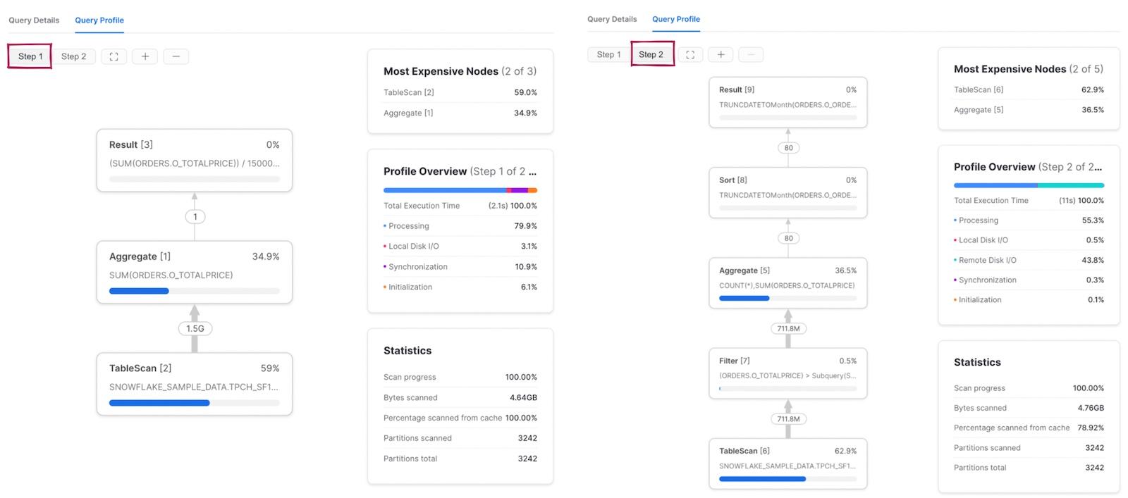
When we modify the filter in the query above to contain a subquery, we end up with a multi-step query.

select
    date_trunc('month', o_orderdate) as order_month,
    count(*) as num_orders,
    sum(o_totalprice) as total_order_value
from snowflake_sample_data.tpch_sf1000.orders
where
    o_totalprice > (select avg(o_totalprice) from snowflake_sample_data.tpch_sf1000.orders)
group by order_month
order by order_month

Unlike above, the query plan now contains two steps. First, Snowflake executes the subquery and calculates the average o_totalprice. The result is stored, and used in the second step of the query which has the same 5 operators as our query above.

Complex Query

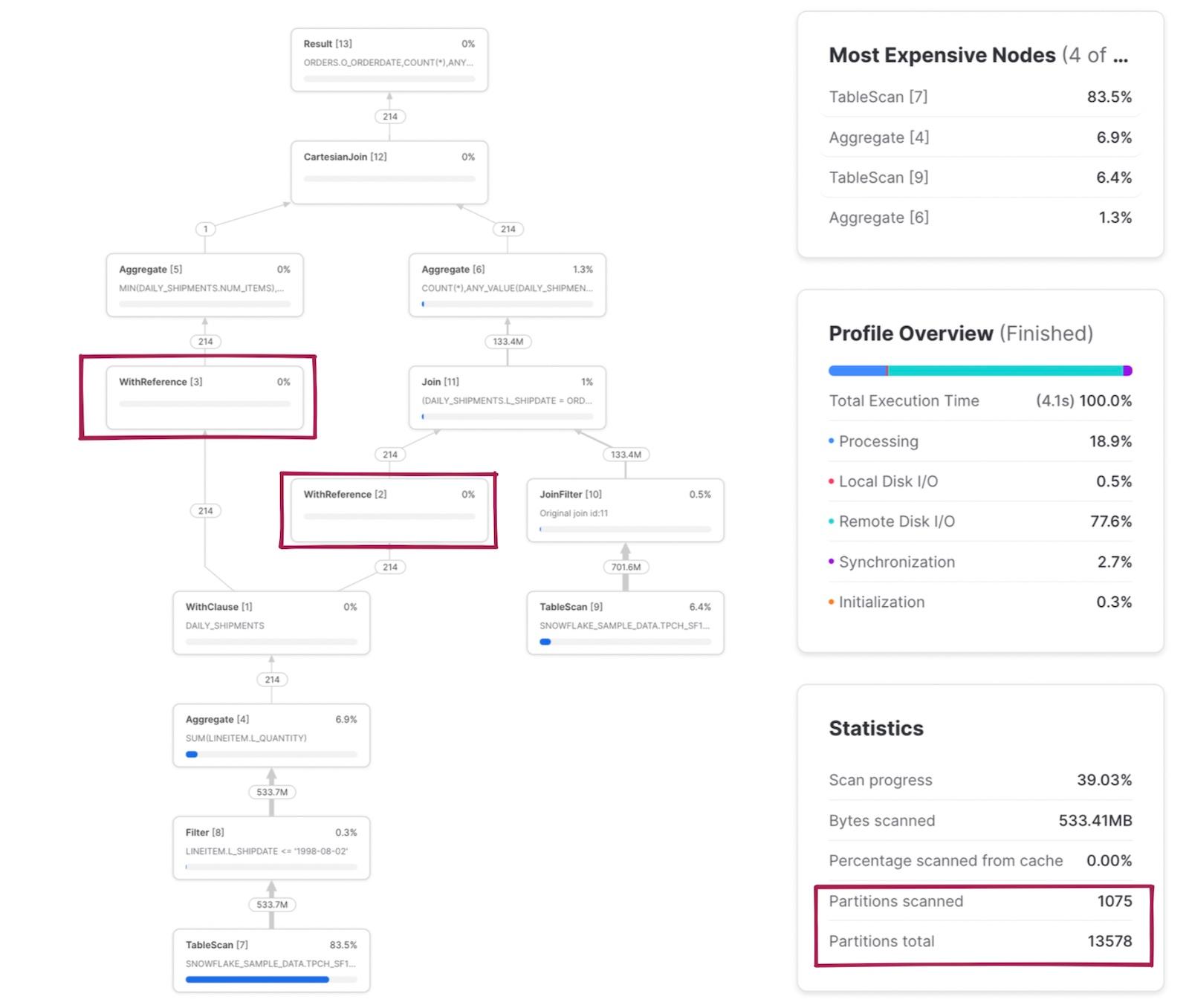
Here is a slightly more complex query ² with multiple CTEs, one of which is referenced in two other places.

with
daily_shipments AS (
    select
        l_shipdate,
        sum(l_quantity) AS num_items
    from snowflake_sample_data.tpch_sf1000.lineitem
    where
        l_shipdate >= DATE'1998-01-01'
        and l_shipdate <= DATE'1998-08-02'
    group by 1
),
daily_summary as (
    select
        o_orderdate,
        count(*) AS num_orders,
        any_value(num_items) AS num_items
    from snowflake_sample_data.tpch_sf1000.orders
    inner join daily_shipments
        on orders.o_orderdate=daily_shipments.l_shipdate
    group by 1
),
summary_stats as (
    select
        min(num_items) as min_num_items,
        max(num_items) as max_num_items
    from daily_shipments
)
select
    daily_summary.*,
    summary_stats.*
from daily_summary
cross join summary_stats

There are a few things worth noting in this example. First, the daily_shipments CTE is computed just once. Any downstream SQL that references this CTE calls the WithReference operator to access the results of the CTE rather than re-calculating them each time.

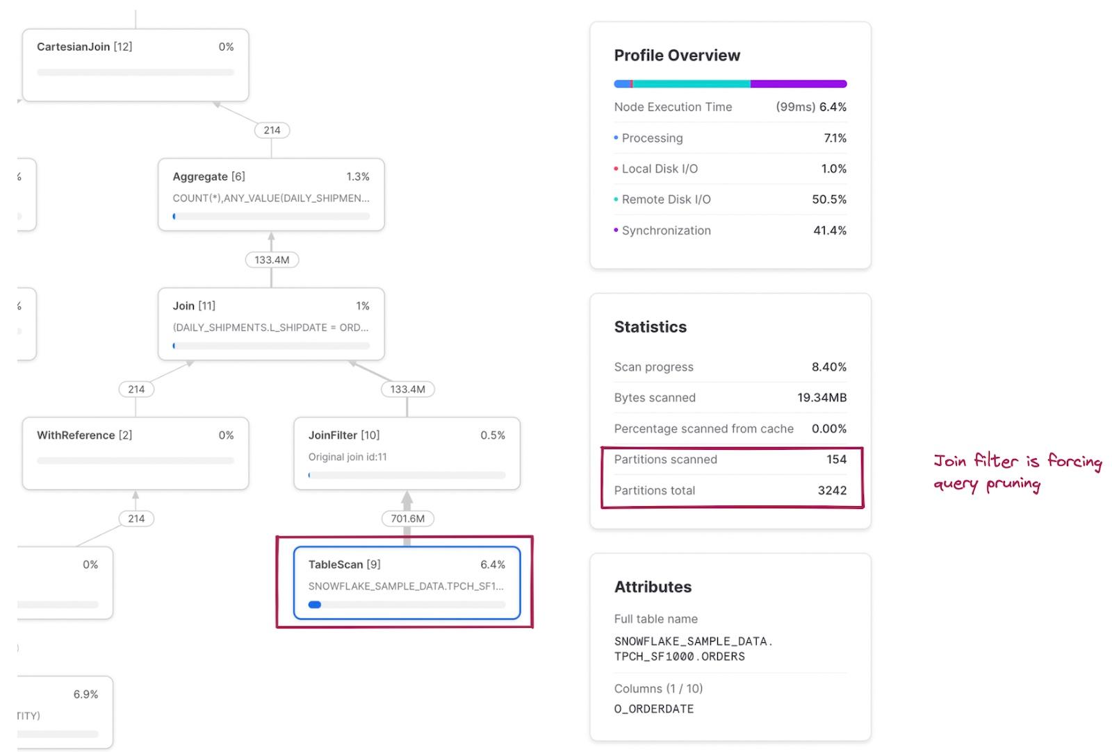
The scanned/total partitions metric is now a combination of both tables being read in the query. If we click into the TableScan node for the snowflake_sample_data.tpch_sf1000.orders table, we can see that the table is being pruned well, with only 154 out of 3242 partitions being scanned. How is this pruning happening when there was no explicit where filter written in the SQL? This is the JoinFilter operator in action. Snowflake automatically applies this neat optimization where it determines the range of dates from the daily_shipments CTE during the query execution, and then applies those as a filter to the orders table since the query uses an inner join!

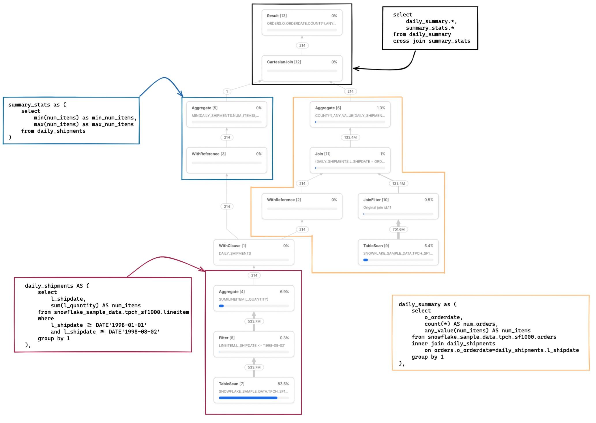
A full mapping of the SQL code to the relevant operator nodes can be found in the notes below ³.

What are things to look for in the Snowflake Query Profile?

The most common use case of the Query Profile is to understand why a particular query is not performing well. Now that we've covered the foundations, here are some indicators you can look for in the Query Profile as potential culprits of poor query performance:

1. High spillage to remote disk. As soon as there is any data spillage, it means your warehouse does not have enough memory to process the data and must temporarily store it elsewhere. Spilling data to remote disk is extremely slow, and will significantly degrade your query performance.
2. Large number of partitions scanned. Similarly to spilling data to remote disk, reading data from remote disk is also very slow. A large number of partitions scanned means your query has to do a lot of work reading remote data.
3. Exploding joins. If you see the number of rows coming out of a join increase, this may indicate that you have incorrectly specificied your join key. Exploding joins generally take longer to process, and lead to other issues like spilling to disk.
4. Cartesian joins. Cartesian joins are a cross-join, which produce a result set which is the number of rows in the first table multiplied by the number of rows in the second table. Cartesian joins can be introduced unintentionally when using a non equi-join like a range join. Due to the volume of data produced, they are both slow and often lead to out-of-memory issues.
5. Downstream operators blocked by a single CTE. As discussed above, Snowflake computes each CTE once. If an operator relies on that CTE, it must wait until it is finished processing. In certain cases, it can be more beneficial to repeat the CTE as a subquery to allow for parallel processing.
6. Early, unnecessary sorting. It's common for users to add an unneeded sort early on in their query. Sorts are expensive, and should be avoided unless absolutely necessary.
7. Repeated computation of the same view. Each time a view is referenced in a query, it must be computed. If the view contains expensive joins, aggregations, or filters, it can sometimes be more efficient to materialize the view first.
8. A very large Query Profile with lots of nodes. Some queries just have too much going on and can be vastly improved by simplifying them. Breaking apart a query into multiple, simpler queries is an effective technique.

In future posts, we'll dive into each of these signals in more detail and share strategies to resolve them.

Notes

¹ Not all 1.3 million records are sent at once. Snowflake has a vectorized execution engine. Data is processed in a pipelined fashion, with batches of a few thousand rows in columnar format at a time. This is what allows an XSMALL warehouse with 16GB of RAM to process datasets much larger than 16GB. ↩

² I wouldn't pay too much attention to what this query is calculating or the way it's written. It was created solely for the purpose of yielding an interesting example query profile. ↩

³ For readers interested in improving their ability to read Snowflake Query Profiles, you can use the example query from above to see how each CTE maps to the different sections of the Query Profile.