Snowflake has skyrocketed in popularity over the past 5 years and firmly planted itself at the center of many companies' data stacks. Snowflake came into existence in 2012 with a unique architecture, described in their seminal white paper as "the elastic data warehouse". Rather than have compute and storage coupled on the same machine like their competitors did ¹, they proposed a new design that took advantage of the near-infinite resources available in cloud computing platforms like Amazon Web Services (AWS). In this post, we'll dive into the three layers of Snowflake's data warehouse architecture ²: cloud services, compute and storage.

Cloud Services

The cloud services layer is the entry point for all interactions a user will have with Snowflake. It consists of stateless services, backed by a FoundationDB database storing all required metadata. Authentication and access control (who can access Snowflake and what can they do within it) are examples of services in this layer. Query compilation and optimization are other critical roles handled by cloud services. Snowflake performs performance optimizations like reducing the number of micro-partitions that a given user's query needs to scan (compile-time pruning).

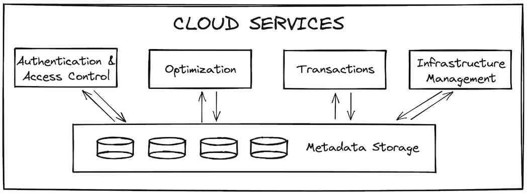
Cloud services are also responsible for infrastructure and transaction management. When new virtual warehouses need to be provisioned to serve a query, cloud services will ensure they become available. If a query is attempting to access data that is being updated by another transaction, the cloud services layer waits for the update to complete before results are returned.

From a performance standpoint, one of the most important roles of cloud services is to cache query results in its global result cache, which can be returned extremely quickly if the same query is run again ³. This can greatly reduce the load on the compute layer ⁴, which we'll discuss next.

Compute

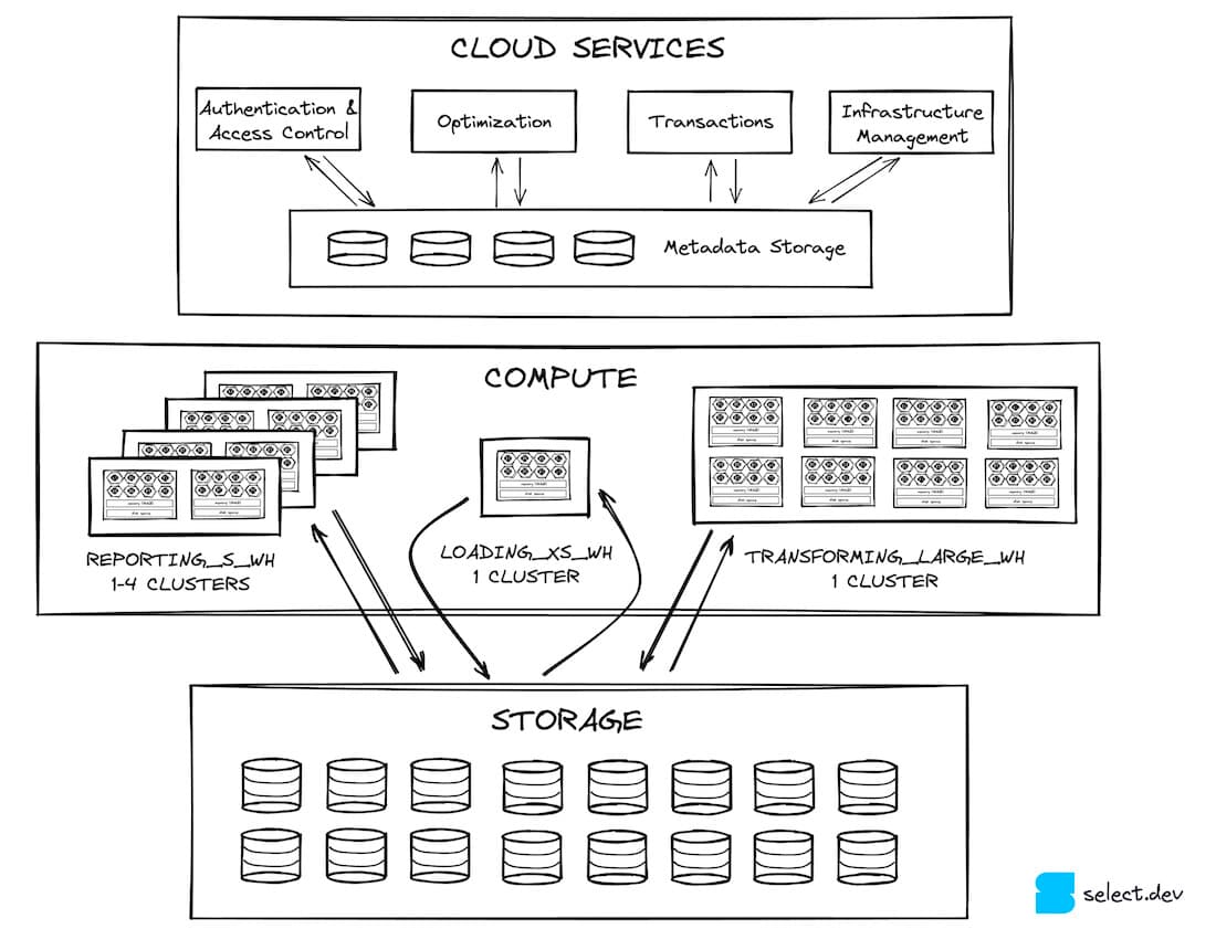
After a given query has passed through cloud services, it is sent to the compute layer for execution. The compute layer is composed of all virtual warehouses a customer has created. Virtual warehouses are an abstraction over one or more compute instances, or "nodes". For Snowflake accounts running on Amazon Web Services, a node would be equivalent to a single EC2 instance. Snowflake uses t-shirt sizing for its warehouses to configure how many nodes they will have. Customers will typically create separate warehouses for different workloads. In the image below, we can see a hypothetical setup with 3 virtual warehouses: a small warehouse used for business intelligence ⁵, an extra-small warehouse used for loading data into Snowflake, and a large warehouse used for data transformations.

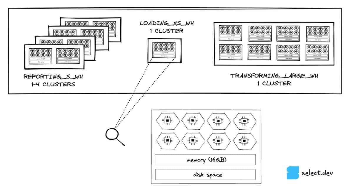
If we zoom in on the extra-small warehouse, the smallest size warehouse offered by Snowflake, we can see that it consists of a single node. Each node has 8 cores/threads, 16GB of memory (RAM), and an SSD cache ⁶, with the exception of 5XL and 6XL which run on different node specifications. With each warehouse size increase, the number of nodes in the warehouse will double. This means that the number of threads, memory, and disk space will also double. A size small warehouse will have twice as much memory (32GB), twice as many cores (16) and double the amount of disk space that an extra-small warehouse will have. By extension, a large warehouse will have 8 times the resources of an extra-small warehouse.

An important aspect of Snowflake's design is that the nodes in each running warehouse are not used anywhere else. This provides users with a strong performance guarantee that their queries won't be impacted by queries running on other warehouses within an account, giving Snowflake customers the ability to run highly performant and predictable data workloads. This differs from the cloud services layer which is shared across accounts, with less consistent timings, though in practice this is inconsequential.

Storage

Snowflake stores your tables in a scalable cloud storage service (S3 if you are on AWS, Azure Blob for Azure, etc.). Every table ⁷ is partitioned into a number of immutable micro-partitions. Micro-partitions use a proprietary, closed-source file format created by Snowflake. Snowflake aims to keep them around 16MB, heavily compressed ⁸. As a result, there can be millions of micro-partitions for a single table.

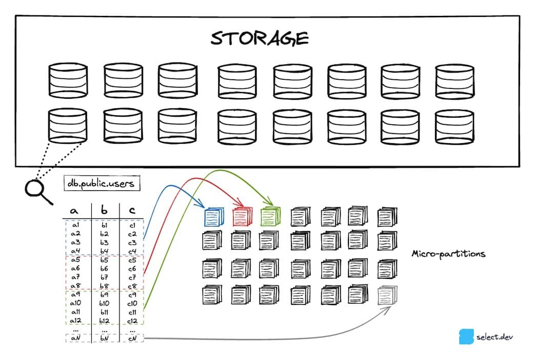
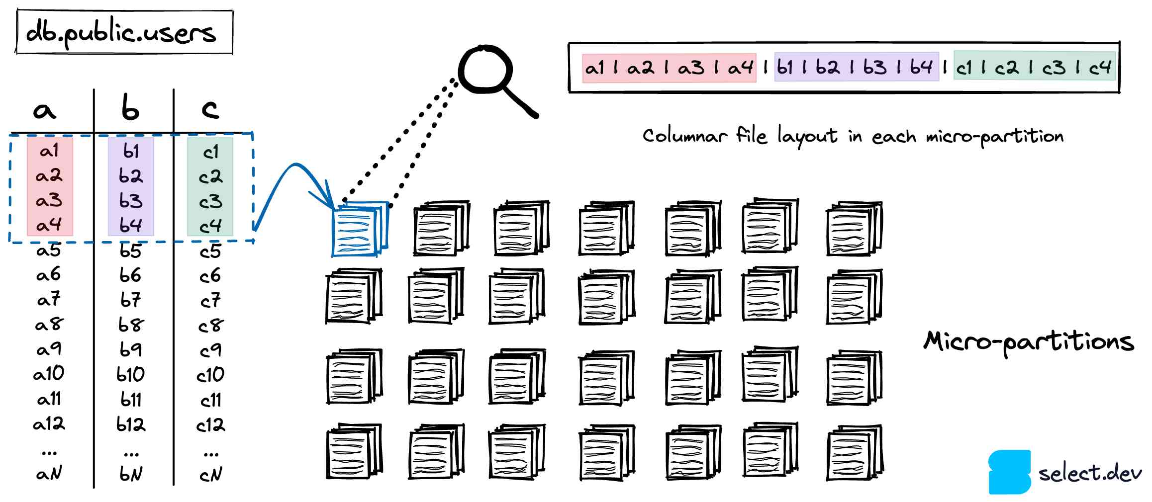
Micro-partitions leverage a columnar storage format instead of a row based layout that is typically used by OLTP databases like Postgres, SQLite, MySql, SQLServer, etc. Since analytical queries typically select a few columns across a wide range of rows, columnar storage formats will achieve significantly better performance.

Column-level metadata is calculated whenever a micro-partition is created. The min/max value, count, # of distinct values, # of nulls are some examples of the metadata that is calculated and stored in cloud services. As discussed earlier, Snowflake can leverage this metadata during query optimization and planning to figure out the exact micro-partitions that must be scanned for a particular query, an important technique known as "pruning". This can vastly speed up queries by eliminating unnecessary, slow data reads.

Because micro-partitions are immutable, DML operations (updates, additions, deletes) must add or remove entire files and re-calculate the required metadata. Snowflake recommends performing DML operations in batches to reduce the number of micro-partitions which are rewritten, which will reduce the total run time and cost of the operations.

Since a table object in Snowflake is essentially a cloud services entry that references a collection of micro-partitions, Snowflake is able to offer innovative storage features like zero-copy cloning and time travel. When you create a new table as a clone of an existing table, Snowflake creates a new metadata entry that points to the same set of micro-partitions. In time travel, Snowflake tracks which micro-partitions a table was comprised of over time, allowing users to access the exact version of a table at a particular point in time.

Summary

Snowflake's unique, scalable architecture has allowed it to quickly become the dominant data warehouse of today. In future posts, we'll dive deeper into each individual layer in Snowflake's architecture and discuss how you can take advantage of their features to maximize query performance and lower costs.

Notes

¹ At the time, Snowflake's main competitors were Amazon Redshift and traditional on-premise offerings like Oracle and Teradata. These existing solutions all coupled storage and compute on the same machines, making them difficult and expensive to scale. Today, Snowflake's bigger competitors are the likes of BigQuery and Databricks. BigQuery likely has a similar market share, if not greater, due to their seamless integration with the rest of their Google Cloud Platform. Databricks has become a new competitor as both companies are beginning to re-position themselves as "data clouds". ↩

² With their move to become a full-on "data cloud", Snowflake is rapidly adding new functionality like Snowpark, Unistore, External Tables, Streamlit and a native App store - all of which extend Snowflake's architecture. We'll be ignoring these new capabilities in this architecture review, and focusing on the data warehousing aspects that most customers use as of today. ↩

³ The queries must be identical in order to be served from the global result cache. In addition, Snowflake actually has two different caches which can benefit performance: a global result cache and a local cache in each warehouse. We'll cover both in more detail in a future post. ↩

⁴ In addition to serving previously run queries from the global result cache, Snowflake can also process certain queries like count(*) or max(column) entirely by leveraging the metadata storage. Learn more in our post about micro-partitions ↩

⁵ This warehouse is actually a multi-cluster warehouse, which means Snowflake will allocate additional compute resources if the query demand surpasses what a single small warehouse can handle. We'll cover multi-cluster warehouses in more depth in a future post. ↩

⁶ These figures are for AWS, and will differ slightly for other cloud providers. They are not guaranteed to be accurate since Snowflake does not publish them, and can change the underlying servers and warehouse configurations at any point. These figures I provided were last validated in August 2022 through two separate sources. Appears to be consistent with what was observed in 2019. I have not been able to validate the disk space available on each node, but plan to figure this out experimentally in the coming months. ↩

⁷ The exception to this is if you are using external tables to store you data. ↩

⁸ This compression is done automatically by Snowflake under the hood. Uncompressed, these files can be over 500MB! ↩