How to speed up range joins in Snowflake by 300x
- Date
 Ian WhitestoneCo-founder & CEO of SELECT
Range joins and other types of non-equi joins are notoriously slow in most databases. While Snowflake is blazing fast for most queries, it too suffers from poor performance when processing these types of joins. In this post we'll cover an optimization technique practitioners can use to speed up queries involving a range join by up to 300x 1.
Before diving into the optimization technique, we'll cover some background on the different types of joins and what makes range joins so slow in Snowflake. Feel free to skip ahead if you're already familiar.
Equi-joins versus non-equi joins
An equi-join is a join involving an equality condition. Most users will typically write queries involving one or more equi-join conditions.
select
  ...
from orders
join customers
  on orders.customer_id=customers.id -- example equi-join condition
A non-equi join is a join involving an inequality condition. An example of this could be finding a list of customers who have purchased the same product:
select distinct
  o1.customer_id,
  o2.customer_id,
  o1.product_id
from orders_items as o1
join orders_items as o2
  on o1.product_id=o2.product_id -- equi-join condition
  and o1.customer_id<>o2.customer_id -- non-equi join condition
Or finding all orders past a particular date for each customer:
select
  ...
from orders
inner join customers
  on orders.customer_id=customers.id
  and orders.created_at > customers.one_year_anniversary_date
What are range joins?
A range join is a specific type of non-equi join. They occur when a join checks if a value falls within some range of values ("point in interval join"), or when it looks for two periods that overlap ("interval overlap join").
Point in interval range join
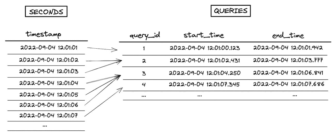
An example of a point in interval range join would be calculating the number of queries running each second:
select
    seconds.timestamp,
    count(queries.query_id) as num_queries
from seconds
left join queries
    on seconds.timestamp between
      date_trunc('second', queries.start_time) and date_trunc('second', queries.end_time)
group by 1
This join could also be based on derived timestamps. For example, find all purchase events which occurred within 24 hours of users viewing the home page:
select
  ...
from page_views
inner join events
  on events.event_type='purchase' -- filter condition
  and page_views.pathname = '/' -- filter condition
  and page_views.user_id=events.user_id -- equi-join condition
  and page_views.viewed_at < events.event_at -- range join condition
  and dateadd('hour', 24, page_views.viewed_at) >= events.event_at -- range join condition
Interval overlap range join
Interval overlap range joins are when a query tries to match overlapping periods. Imagine that for each browsing session on your landing page site you need to find all other sessions that occurred at the same time in your application:
select
    s1.session_id,
    array_agg(s2.session_id) as concurrent_sessions
from landing_page_sessions as s1
inner join app_sessions as s2
   on s1.end_time > s2.start_time
   and s1.start_time < s2.end_time
group by 1
Why are range joins slow in Snowflake?
Range joins are slow in Snowflake because they get executed as cartesian joins with a post filter condition. A cartesian join, also known as a cross join, returns the cartesian product of the records between the two datasets being joined. If both tables have 10 thousand records, then the output of the cartesian join will be 100 million records! Practitioners often refer to this as a join explosion 💥. Query execution can be slowed down significantly when Snowflake has to process these very large intermediate datasets.
Let's use the "number of queries running per second" example from above to explore this in more detail.
select
    s1.session_id,
    array_agg(s2.session_id) as concurrent_sessions
from landing_page_sessions as s1
inner join app_sessions as s2
   on s1.end_time > s2.start_time
   and s1.start_time < s2.end_time
group by 1
Our seconds table contains 1 row per second, and the queries table has 1 row per query. The goal of this query is to lookup which queries were running each second, then aggregate and count.
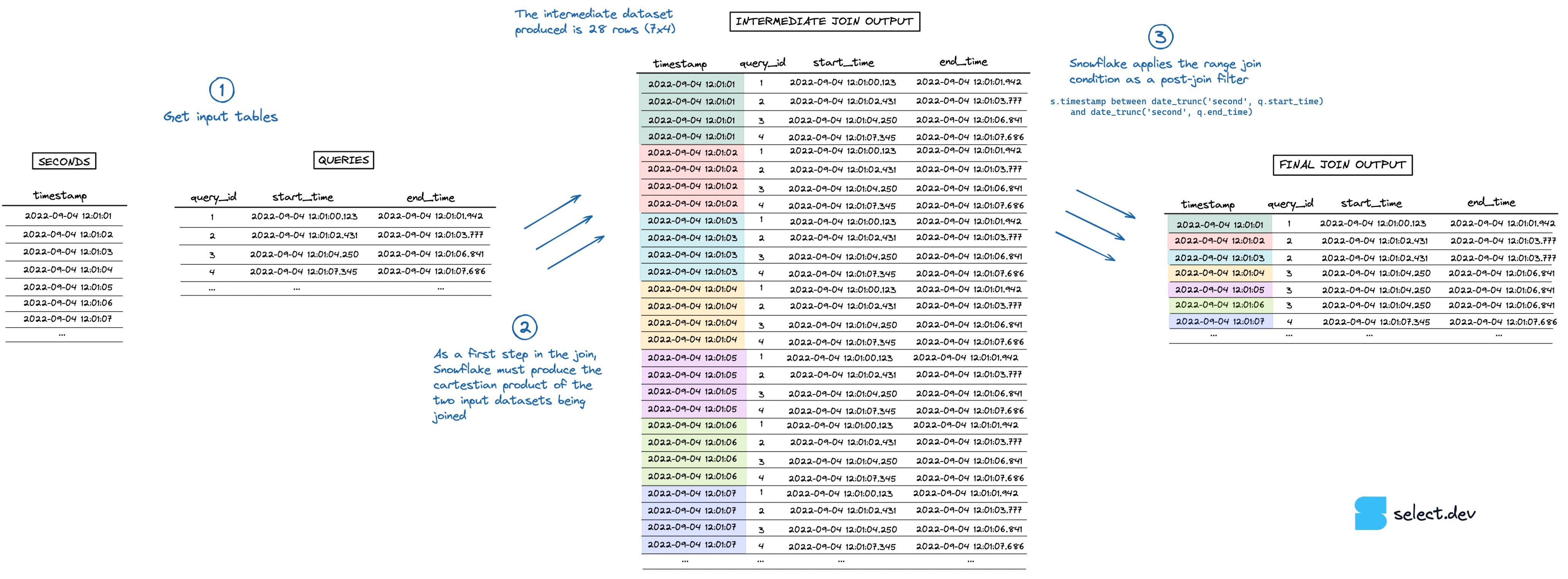
When executing the join, Snowflake first creates an intermediate dataset that is the cartesian product of the two input datasets being joined. In this example, the seconds table is 7 rows and the queries tables is 4 rows, so the intermediate dataset explodes to 28 rows. The range join condition that performs the "point in interval" check happens after this intermediate dataset is created, as a post-join filter. You can see a visualization of this process in the image below (go here for a full screen, higher resolution version).

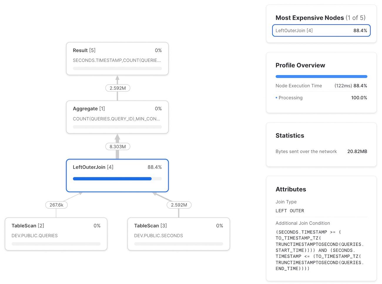
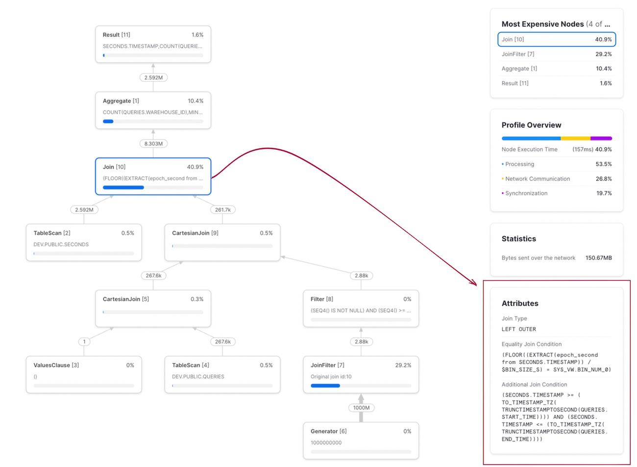
Running this query on a 30 day sample of data with 267K queries took 12 minutes and 30 seconds. As shown in the query profile, the join is the clear bottleneck in this query. You can also see the range join condition expressed as an "Additional Join Condition":
How to optimize range joins in Snowflake
When executing range joins, the bottleneck for Snowflake becomes the volume of data produced in the intermediate dataset before the range join condition is applied as a post-join filter. To accelerate these queries, we need to find a way to minimize the size of the intermediate dataset. This can be accomplished by adding an equi-join condition, which Snowflake can process very quickly using a hash join. 2
Minimize the row explosion
While the principle behind this is intuitive, make our datasets smaller, it is tricky in practice. How can we constrain the intermediate dataset prior to applying the range join post-join filter? Continuing with the queries per second example from above, it is tempting to add an equi-join condition on something like the hour of each timestamp:
select
    seconds.timestamp,
    count(queries.query_id) as num_queries
from seconds
left join queries
    on date_trunc('hour', seconds.timestamp)=date_trunc('hour', queries.start_time) -- NEW: equi-join condition
    and seconds.timestamp -- range join condition
      between date_trunc('second', queries.start_time) and date_trunc('second', queries.end_time)
group by 1
Promising, but the approach falls apart when the interval (query total run time) is greater than 1 hour. Because the equi-join is on the hour the query started in, all records in any subsequent hours wouldn't be counted.
This can be solved by creating an intermediate dataset, query_hours, containing 1 row per query per hour the query ran in. It then becomes safe to join on hour, since we'll have 1 row for each hour the query ran. No records get inadvertently dropped.
with
query_hours as (
  select
    queries.*,
    hours_list.timestamp as query_hour
  from queries
  inner join hours_list -- dataset containing 1 row per hour
    on hours_list.timestamp between date_trunc('hour', queries.start_time) and date_trunc('hour', queries.end_time)
)
select
    seconds.timestamp,
    count(queries.query_id) as num_queries
from seconds
left join query_hours as queries
    on date_trunc('hour', seconds.timestamp)=queries.query_hour -- NEW: equi-join condition
You might have noticed that the query_hours CTE involves a range join itself - won't that be slow? When applied for the right queries, the additional time spent on the input dataset preparation will result in a much faster query overall
3. Another concern may be that the query_hours dataset becomes much larger than the original queries dataset, as it fans out to 1 row per query per hour. Since most queries finish in well under 1 hour, the query_hours dataset will be similar in size to the original queries dataset.
Adding the new equi-join condition on hours helps accelerate this range join query by constraining the size of the intermediate dataset. However, this approach is not ideal for a few reasons. Maybe hour isn't the best choice, and something else should be used as a constraint. Additionally, how can this approach be extended to support range joins involving other numeric datatypes, like integers and floats?
Binned range join optimization
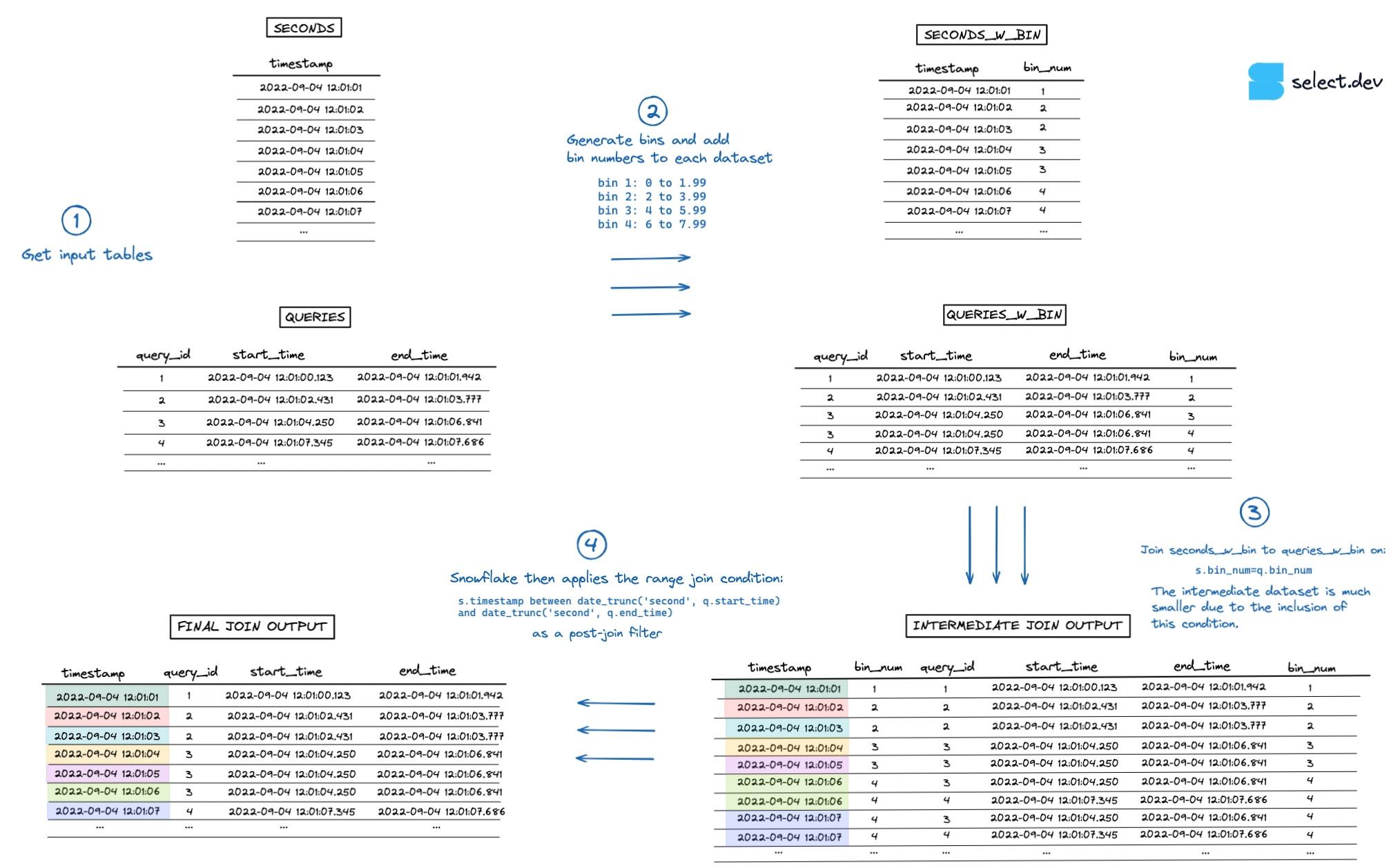
We can extend the ideas from above into a more generic approach via the use of 'bins' 4.
By telling Snowflake to only apply the range join condition on smaller subsets of data, the join operation is much faster. For each timestamp, Snowflake now only joins queries that ran in the same hour, instead of every query from all time.
Instead of limiting ourselves to predefined ranges like "hour", "minute" or "day", we can instead use arbitrarily sized bins. For example, if most queries run in under 2 seconds, we could bucket the queries into bins that span 2 seconds each.
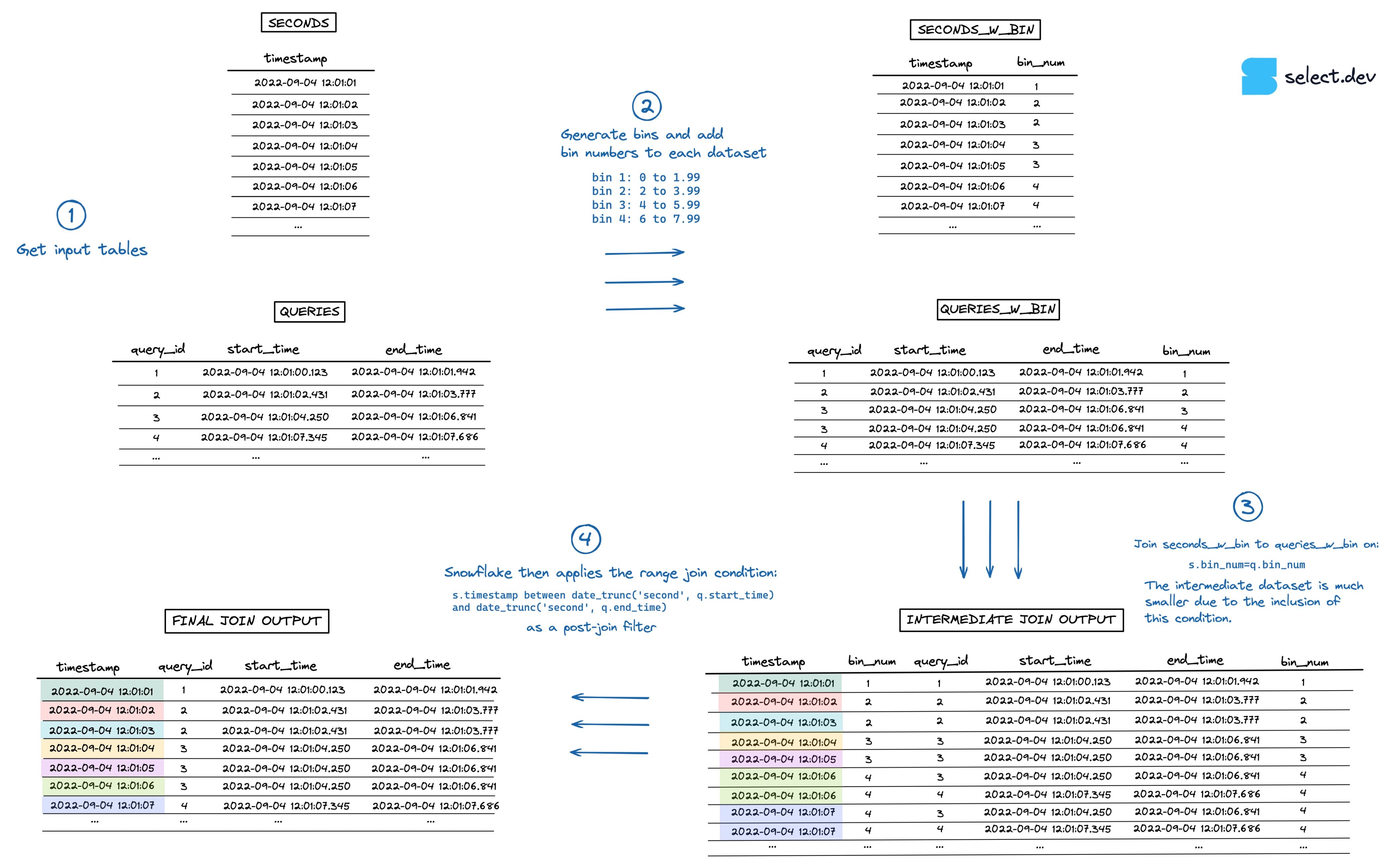
The algorithm would look something like this:
- Generate the bins and add bin numbers to each dataset
- Add the equi-join condition constraint to the range join using
bin_num, similar to what was done above withhour. - The intermediate dataset created is now much smaller.
- As usual, Snowflake applies the range join as a post-join filter. This time, much faster.
You can see a visualization of this process in the image below (go here for a full screen, higher resolution version).
Example binned range join query
Bin numbers are just integers that represent a range of data. One way to create them is to divide the number by the desired bin size. With timestamps, we can first convert the timestamp to unix time, which is an integer, before dividing:
-- for 60 second sized bins
select
  timestamp,
  floor(date_part(epoch_second, timestamp) / 60) as bin_num
We'll save this in a function, get_bin_number
5, to avoid repeating it each time.
Following the steps described above, we first need to generate the list of applicable bins. This is accomplished by using a generator to create a list of integers, then filtering that list down to the desired start and end bin numbers 6.
set bin_size_s = 60;

with
metadata as (
    select
        -- this would be a query against your desired time range
        min(timestamp) as start_time,
        max(timestamp) as end_time,
        get_bin_number(start_time, $bin_size_s) as bin_num_start,
        get_bin_number(end_time, $bin_size_s) as bin_num_end
    from seconds
),
-- need a CTE with 1 row between bin_num_start and bin_num_end
-- have to first generate a massive list, then filter down since you can't pass in calculated values
-- when bins_base is 1 trillion takes 5 seconds to filter down. 106 ms for for 1 million
Now we can add the bin number to each dataset. For the queries dataset, we'll output a dataset with 1 row per query per bin that the query ran within. For the seconds dataset, each timestamp will be mapped to a single bin.
queries_w_bin_number as (
    select
        start_time,
        end_time,
        warehouse_id,
        cluster_number,
        bins.bin_num
    from queries
    inner join bins
        on bins.bin_num between
          get_bin_number(queries.start_time, $bin_size_s) and get_bin_number(queries.end_time, $bin_size_s)
),
seconds_w_bin_number as (
    select
        timestamp,
And apply the final join condition, with the added equi-join condition on bin_num:
select
    s.timestamp,
    count(q.warehouse_id) as num_queries
from seconds_w_bin_number as s
left join queries_w_bin_number as q
    on s.bin_num=q.bin_num
    and s.timestamp between date_trunc('second', q.start_time) and date_trunc('second', q.end_time)
group by 1
Using the same dataset as above, this query{% superscript id=7 /%} executed in 2.2 seconds, whereas the un-optimized version from earlier took 750 seconds. That's over a 300x improvement. The query profile is shown below. Note how the join condition now shows two sections: one for the equi-join condition on bin_num, and another for the range join condition.
Choosing the right bin size
A key part of making this strategy work involves picking the right bin size. You want each bin to contain a small range of values, in order to minimize row explosion in the intermediate dataset before the range join filter is applied. However, if the bin size you pick is too small, the size of your "right table" (queries) will increase significantly when you fan it out to 1 row per bin.
According to databricks, a good rule of thumb is to pick the 90th percentile of your interval length. You can calculate this using the approx_percentile function along with DATEDIFF. I've shown the values for the queries sample dataset I've been using throughout this post.
select
    approx_percentile(datediff('second', start_time, end_time), 0.5) as p50, -- 2s
    approx_percentile(datediff('second', start_time, end_time), 0.90) as p90, -- 30s
    approx_percentile(datediff('second', start_time, end_time), 0.95) as p95, -- 120s
    approx_percentile(datediff('second', start_time, end_time), 0.99) as p99, -- 600s
    approx_percentile(datediff('second', start_time, end_time), 0.999) as p999, -- 900s
    count(*) -- 267K
from queries
Rules of thumb are not perfect. If possible, test your query with a few different bin sizes and see what performs best. Here's the performance curve for the query above, using different bin sizes. In this case, picking the 99.9th percentile versus the 90th percentile didn't make much of a difference. As expected, query times started to get worse once the bin size got really small.

How to extend to a join with a fixed interval?
- Explain how this would be extended to a fixed interval point in interval join
- Bin size would be set to fixed interval size
If you have a point in interval range join with a fixed interval size, like the query shared earlier:
select
  ...
from page_views
inner join events
  on events.event_type='purchase' -- filter condition
  and page_views.pathname = '/' -- filter condition
  and page_views.user_id=events.user_id -- equi-join condition
  and page_views.viewed_at < events.event_at -- range join condition
  and dateadd('hour', 24, page_views.viewed_at) >= events.event_at -- range join condition
Then set your bin size to the size of the interval: 24 hours.
How to extend to an interval overlap range join?
If you are dealing with an interval overlap range join, like the one shown below:
select
    s1.session_id,
    array_agg(s2.session_id) as concurrent_sessions
from landing_page_sessions as s1
inner join app_sessions as s2
   on s1.end_time > s2.start_time
   and s1.start_time < s2.end_time
group by 1
You can apply the same binned range join technique after you've fanned out both landing_page_sessions and app_sessions to contain 1 row per session per bin the session fell within (as was done with queries above).
When should this optimization be used?
As a first step, ensure that the range join is actually a bottleneck by using the Snowflake query profile to validate it is one of the most expensive nodes in the query execution. Adding the binned range join optimization does make queries harder to understand and maintain.
The binned range join optimization technique only works for point in interval and interval overlap range joins involving numeric types. It will not work for other types of non-equi joins, although you can apply the same principle of trying to add an equi-join constraint wherever possible to reduce the row explosion.
If the dataset on the "right", with the start and end times, contains a relatively flat distribution of interval sizes, then this technique won't be as effective.
Notes
1This stat is from a single query, so take it with a handful of salt. Your mileage will vary depending on many factors. ↩
2This approach was inspired by Simeon Pilgrim's post from 2016 (back when Snowflake was snowflake.net!). I used it quite successfully until implementing the more generic binning approach. ↩
3The range join to the hours table will be much quicker than the range join to the seconds table, since the intermediate table will be ~3600 times smaller.
↩
4This approach was inspired by Databricks. They don't go into the details of how their algorithm is implemented, but I assume it works in a similar fashion. ↩
5Optionally create a get_bin_number function to avoid copying the same calculation throughout the query:
create or replace function get_bin_number(timestamp timestamp_tz, bin_size_s integer)
  returns integer
  as
  $$
    floor(date_part(epoch_second, timestamp) / bin_size_s)
  $$
6Snowflake doesn't let you pass in calculated values to the generator, so this had to be done in a two step process. In the near future we'll be open sourcing some dbt macros to abstract this process away. ↩
7The full example binned range join optimization query:
create or replace function get_bin_number(timestamp timestamp_tz, bin_size_s integer)
  returns integer
  as
  $$
    floor(date_part(epoch_second, timestamp) / bin_size_s)
  $$
;

set bin_size_s = 60;

with
metadata as (
    select
        -- Get the time range your query will span
        min(timestamp) as start_time,
Ian is the Co-founder & CEO of SELECT, a SaaS Snowflake cost management and optimization platform. Prior to starting SELECT, Ian spent 6 years leading full stack data science & engineering teams at Shopify and Capital One. At Shopify, Ian led the efforts to optimize their data warehouse and increase cost observability.
Get up and running with SELECT in 15 minutes.
Snowflake optimization & cost management platform
Gain visibility into Snowflake usage, optimize performance and automate savings with the click of a button.