At the heart of the heavy lifting we all do in Snowflake sits the Virtual Warehouse. A Virtual Warehouse as an abstraction on top of commodity compute, such as EC2 in AWS or VMs in Azure. When you run a query, Snowflake instantly provisions these compute nodes to do the work.

Recently, Snowflake rolled out a major update to the Virtual Warehouses called Generation 2 (Gen2) Warehouses. Gen2 warehouses represent a significant improvement over the traditional Standard Virtual Warehouse.

What are Snowflake Gen2 Standard Warehouses?

Gen2 warehouses take advantage of faster hardware made available from the underlying cloud providers (AWS, GCP). In addition, the Snowflake team has invested in specific software optimizations on Gen2 warehouses that will yield additional performance and cost improvements. Almost all queries will see a performance gain from the underlying hardware improvements, but specific workloads will see additional improvements from the software optimizations.

Gen2 Warehouses currently have limited availability, but we expect they will be released in more regions very quickly. Check here to see if Gen2 is available in your region.

Hardware Improvements

Gen2 virtual warehouses in Snowflake run on your cloud provider’s compute infrastructure, such as EC2 instances or virtual machines. Over time, these cloud providers upgrade their instances with newer hardware. AWS, for example, recently introduced Graviton4 ARM-based processors. While Snowflake does not disclose the specific hardware it uses, it’s reasonable to assume they are leveraging the latest offerings from each provider. These hardware improvements include faster local disk reads, enhanced CPU performance, and higher network throughput, all of which contribute to better out-of-the-box query performance.

Software Improvements

Snowflake has also reported making a number of software specific optimizations which will help accelerate DML workloads (i.e. jobs that merge / update data in tables) as well as certain complex queries.

As we’ll see in the results of our analysis, these software improvements are likely the cause behind some of the larger performance gains.

How are Gen2 Warehouses priced?

Since Gen2 warehouses run on newer, better hardware, they are more expensive. As you can see in the pricing table below (source), Gen2 warehouses are 35% more expensive in AWS and GCP, and 25% more expensive in Azure.

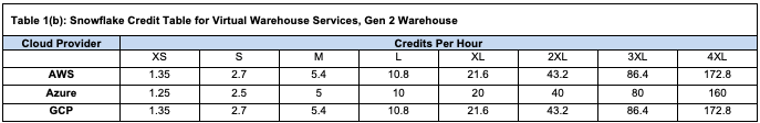
This has significant implications that every practitioner should consider before switching. Even if queries run quicker, you’ll need to ensure the decreased compute time offsets the increased cost. To further complicate the matter, most practitioners configure warehouses to suspend after 60 seconds of idle time. This means you will be incurring the higher cost during the idle time and you may want to factor that in to your analysis.

Break Even Calculation

Since the queries run faster on Gen2 and you are billed the higher rate for less time, the break even calculation is:

Required Time Reduction (%) = 1 - (1 / Price Increase Factor)

In Azure, 20% reduction in warehouse up time is required to break even.

• 1 - (1 / 1.25) = 0.20

In AWS, 25.9% reduction in warehouse up time is required to break even.

• 1 - (1 / 1.35) = 0.259

Don’t forget the 1 minute minimum billing period

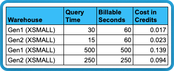
Keep in mind that every time a warehouse resumes you are billed for 60 seconds. So if you have a query that goes from 30 seconds in Gen1 and 15 seconds in Gen2, you are not saving any money - you’re paying more. It’s up to you to decide whether the performance improvements are worth the added costs.

The ideal savings scenario: workloads that run more than 1 minute AND save more than the break even percent above.

The table below summarizes this concept.

How to create a Snowflake Gen2 Warehouse

Creating a new Gen2 warehouse, or converting an existing warehouse to Gen2 is very simple: Just pass the resource_constraint parameter to the create or alter statement. Here is an example of each:

-- create new
CREATE OR REPLACE WAREHOUSE my_wh
WAREHOUSE_SIZE = MEDIUM
RESOURCE_CONSTRAINT = STANDARD_GEN_2;

-- alter existing
ALTER WAREHOUSE legacy_wh 
SET RESOURCE_CONSTRAINT = STANDARD_GEN_2;

Benchmarking Data

Snowflake comes with a sample database containing the TCP-H dataset. TCP-H is a dataset defined by Transaction Processing Performance Council for benchmarking analytical workloads.

In Snowflake, you will find these schemas in the snowflake_sample_data database:

• TPCH_SF1
• TPCH_SF10
• TPCH_SF100
• TPCH_SF1000

The SF stands for Scale Factor. SF10 is 10x larger than SF1, and so on. We tested various types of workloads on each of SF10, SF100, and SF1000.

Benchmarking Scenarios

We covered three main scenarios for benchmarking:

1. dbt: Building a dbt project that consists entirely of Table models and tests. The purpose of this to see if dbt projects, which are widely used on Snowflake, are good candidates for Gen2 warehouses.
2. Select queries: Here, we are mimicking what would happen in a BI tool or other user facing applications.
3. DML workloads: updating / merging new data into Snowflake is a common workload for data engineerings teams. We tested various DML scenarios (updates, merges, etc.) to understand how they were impacted.

Benchmarking Results

dbt

Setup

We forked and updated a dbt existing project that works with the Snowflake TCPH datasets. Our repo can be found here.

We ran the dbt project wide open against each data set using warehouses of various sizes and compared Gen1 vs Gen2. We used smaller warehouses on smaller data and bigger warehouses on bigger data, to simulate a realistic scenario.

Each iteration was built in a fresh schema to avoid caching and to persist the results of each test separately. Each build runs 16 table models and 43 data tests. (dbt build --exclude tag:merge-test ).

Results

Here were the results:

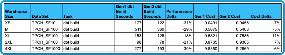
The work done in this dbt project amounts to roughly 97% CTAS queries (table models), and 3% dbt tests (simple select queries).

Based on this, for dbt’s table models in this specific project, the performance gain is not always high enough to justify the extra 35% cost.

It is also worth noting that the 4XL Gen2 warehouse had a very long cold start time, upwards of 5 minutes, whereas the Gen1 4XL started up right ways. Since you are not billed for the warehouse resume time, we removed that from the result by pre-starting the warehouse prior to running dbt. Warehouse provisioning times are usually not an issue for ETL jobs which run overnight, but worth noting.

Simple select statements

We ran a sample of select queries from the TPCH datasets to simulate what would happen in a BI tool or other user facing applications. The exact queries run are linked in the table. Here were the results:

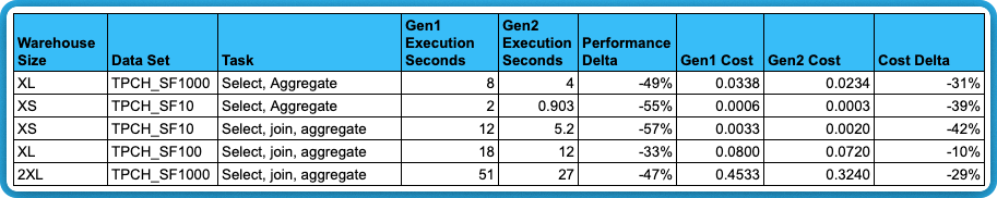
These select statements show great performance gains and all of them save money on Gen2 on a per second basis. It’s worth noting that since these user facing queries must be fast, we are now faced with the minimum billing period nuance from Snowflake. If queries are running less than 60 seconds and/or the warehouse is sitting idle for extended periods (which is common in BI tools), Gen1 is still recommended, unless you care optimizing specifically for speed and can absorb the added costs.

It’s also worth mentioning that Gen2 warehouses open up the door for dropping your warehouse size. For example, if you cut query times in half with Gen2 warehouses, but the costs go up due to idle time becoming more expensive, you could arguably drop your warehouse size in half, get the same query performance at a lower cost, and experience significant cost savings.

DML: Update large tables

The updates in this section are all simple updates based on update table <tbl> set column <col> = value. Note, even though we are updating a single column, Snowflake will have to re-write the entire micro-partition for that given row. So effectively, these two commands require the same amount of “work” from Snowflake:

update orders_table set customer_id=5 where order_id=1;
update orders_table set customer_id=5, amount=22.05, order_date='2025-05-01',
<many columns>
where order_id=1;

Here we ran three scenarios:

• An update with no where clause on 6 billion rows.
• Selective update on the same table, where only 2.4 million rows (0.04% of the table) are updated.
• Update a single row.
• The SQLs statements can be found here.

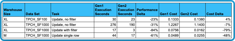
I think the results are pretty conclusive, Gen2 warehouses are very good at filtered updates, likely due to the specific software optimizations Snowflake released.

Let’s analyze the query with -79% cost delta a little deeper to see if we can figure out why there is such a huge improvement.

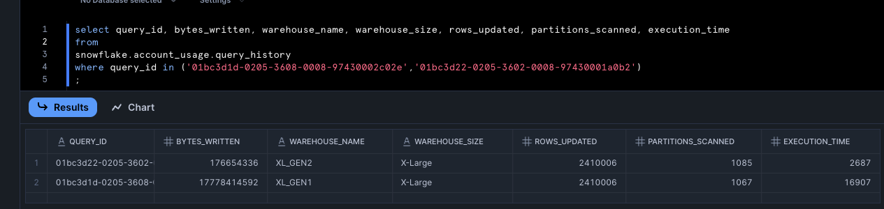
The screenshot shows a 99% reduction in bytes written!

(0.16 GB – 16.56 GB) / 16.56 GB = -99%

DML: Merge queries

Setup

Unlike the simple updates above, the Merge queries updates records in the target based on records in a source. In this case a join is used to update matched records and insert new ones.

The merge queries with n% of rows updated are dbt incremental models. These are run by executing dbt run -s pre_merge+ and editing the row limit filter on line 22. These simulate a real life Incremental situation, where only a fraction of the data is new or updated. To change the % of data updated, we change this line and run the model + downstream incremental model.

The “Merge, all rows updated” tasks come from this query, which updates every row in the data.

Keep in mind, the SF10 data set has about 60 million rows and the SF100 has about 600 Million rows.

Results

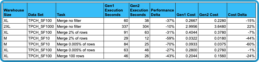
The results above conclusively show that merge queries updating a small number of records experience a greater performance improvement compared to wide-open merges.

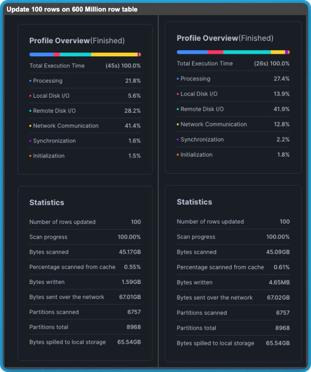
The evidence lies in the query profile, which reveals several notable details. First, network communication dropped significantly from 41% to 13%. This change is likely due to the dramatic reduction in bytes written—from 1.6GB down to just 4.65MB. This suggests that Snowflake may have improved compression or optimized how data is transmitted over the network. Since both queries only update 100 rows, this supports the idea that Gen2 includes specific optimizations for writing data more efficiently.

An anomoly

The one anomaly (on the second to last row, showing only 1% savings) is truly interesting because Snowflake shows that 99.5% fewer bytes were written. There are a few possible explanations for this including S3 throttling and network speed.

Idle Time Considerations

All of our results above are shown on a per-second basis. But as we mentioned earlier, idle time after queries are done running is a consideration. Let’s mock up a simple scenario. In the table below, we assume that Gen2 can run a query in 50% less time than Gen1. A very generous assumption, but let’s keep it simple. Let’s also assume a 60 second auto-suspend is configured. That would give us:

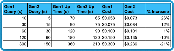
Obviously the longer the workload runs the less impact this has. The table below gives you an idea of how this impact is reduced as query duration increases:

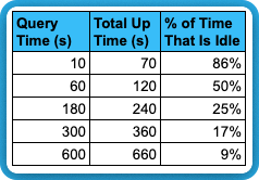
This phenomena can be expressed as a function:

% idle time = [auto suspend seconds] / ([Query Time] + [auto suspend seconds])

For Snowflake Customers who are trying to optimize for performance, the impact of the idle time is negligible compared to the cost of having a data engineer fine tune queries, and spending more credits while doing so! But the idle time should be considered.

Consolidated results and wrap up

Reviewing aggregated results

Reviewing aggregated results can be deceptive because it is heavily influenced by the number of queries we ran in each category and warehouse size. It also hides that specific queries within a category can have vastly different results than the aggregate.

Despite this problem, it is still useful to view the aggregated data because we learn that the cost change and performance is varied.

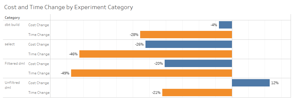
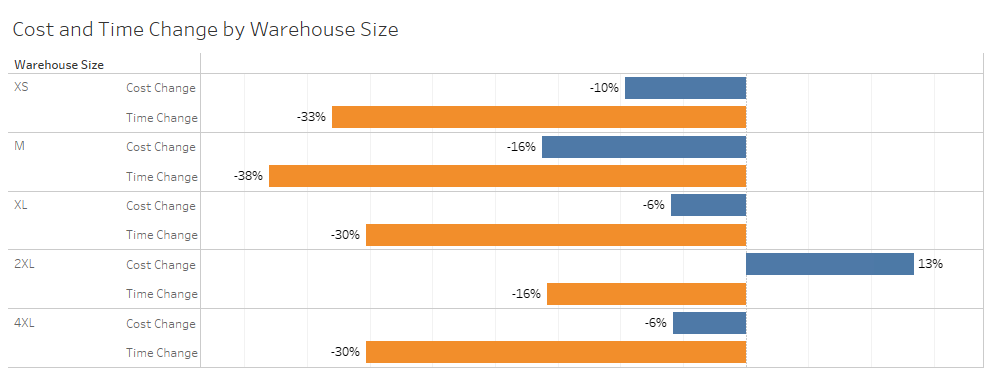
Below you will find the results from the above tests, consolidated for easy review.

I think the lesson here is always experiment with your data set to see how Gen2 is performing for your specific use cases. Just like most things in the cloud, it is really hard to say which tooling is universally cheaper or better. It is always use-case specific.

But, there are a few key takeaways:

• We now have a zero effort knob you can use to speed up queries and usually reduce cost.
• Simple select queries were among the top performers in our tests, saving 26% on cost.
  • However, they may end up being more expensive if running on unsaturated warehouses for less than the minimum billing period.
  • Keep in mind, this may be perfectly fine to pay 10% more (say, an extra $10K/year) for a zero-effort 20% improvement for all your business users. Consider the tradeoffs of how long it would take you to make the performance optimizations yourself.
• Gen2 is head-and-shoulders better than Gen1 for targeted updates and simple select queries involving full table scans.
• Gen2 is not necessarily cheaper for your average dbt table models. This is likely due to the re-writing of all partitions of the data using “create or replace table as”. However, it could be cheaper and faster on incremental models which involve merge statements.

I think a great use case for Gen2 warehouses is when your current warehouse is constrained and you are considering upsizing, let’s say from Medium to Large. Instead of upsizing to Large where the credits cost 100% more, try to upsize to Gen2 Medium instead, and only pay 35% more for each credit. Personally, I’m starting to think of Gen2 as a half increment between each warehouse size.

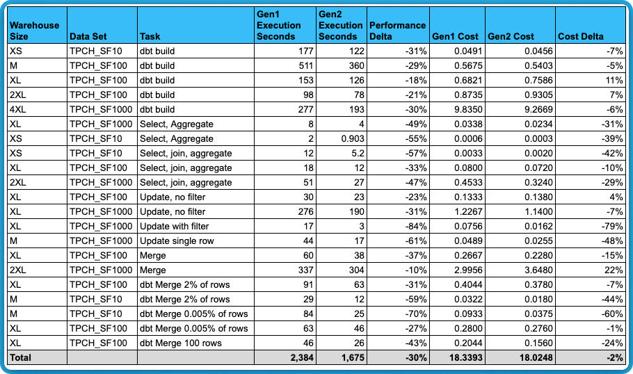
• Total savings was 2% - but this is heavily skewed by the two largest workloads.
• After excluding the two largest credit consumers, total savings is 7%.

Things to keep in mind with benchmarking experiments

When discussing our benchmark results with someone from Snowflake, he stated something that resonated with us: “The only thing a benchmark tells you is how quickly the benchmark ran”. There are a lot of factors to consider in how this will impact your production workload.

• Lack of concurrency: benchmarks for the most part run on unsaturated warehouses where concurrency is not an issue.
• Transient noise: the same query run under the same conditions could vary by about 10% plus or minus if run at another time due to natural variability in the underlying cloud infrastructure (transient issues, AWS S3 service throttling, etc).

We suggest running Gen2 on targeted workloads for a period of time, maybe a week or so, to see the actual cost impact in your environment.

Next Steps

At SELECT, we’d like to build a more robust and scientific approach to benchmarking. We imagine a scenario where python runs the same query multiple times against the same data set using different warehouses. This will allow us to get a larger sample size where each individual result has less impact on the average. Stay tuned for more!

We’re excited to hear from you on your experience with Gen2 warehouses! Please reach out and let us know about any interesting findings or cost savings stories!