In our previous post on Snowflake clustering, we discussed the importance of understanding table usage patterns when deciding how to cluster a table. If a particular field is used frequently in where clauses, that can make a great candidate as a cluster key. But what if there are other frequently used where predicates that could benefit from clustering?

In this post we compare three options:

1. A single table with multi-column cluster keys
2. Maintaining separate tables clustered by each column
3. Using clustered, materialized views to leverage Snowflake's powerful automatic pruning optimization feature

The limitations of multi-column cluster keys

When defining a cluster key for a single table, Snowflake allows you to use more than one column. Let’s say we have an orders table with 1.5 billion records:

-- 1,500,000,000 records
create table orders as (
  select
    o_orderdate,
    o_orderkey,
    o_custkey,
    o_clerk
  from snowflake_sample_data.tpch_sf1000.orders
)

A common scenario goes like this. The finance team regularly query specific date ranges on this table in order to understand our sales volume. We also have our engineering teams querying this table to investigate specific orders. On top of that, marketing wants the ability to see all historical orders for a given customer.

That’s three different access patterns, and as a result, three different columns we’d want to cluster our table by: o_orderdate, o_custkey and o_orderkey. As shown in Snowflake’s documentation, we can define a multi-column cluster key for our table using all three columns in the cluster by expression ¹:

create table orders cluster by (o_orderdate, o_custkey, o_orderkey) as (
  select
    o_orderdate, -- 2,406 distinct values
    o_orderkey, -- 1,500,000,000 distinct values
    o_custkey, -- 99,999,998 distinct values
    o_clerk
  from snowflake_sample_data.tpch_sf1000.orders
)

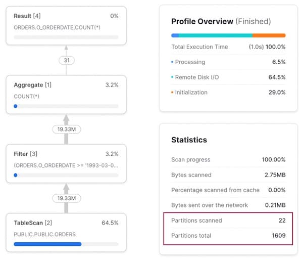
Access Pattern 1: Query by date

select
    o_orderdate,
    count(*) as cnt
from orders
where o_orderdate between '1993-03-01' and '1993-03-31'
group by 1

Running a query against a range of dates, we can see from the query profile that we are getting excellent query pruning. Only 22 out of 1609 micro-partitions are being scanned.

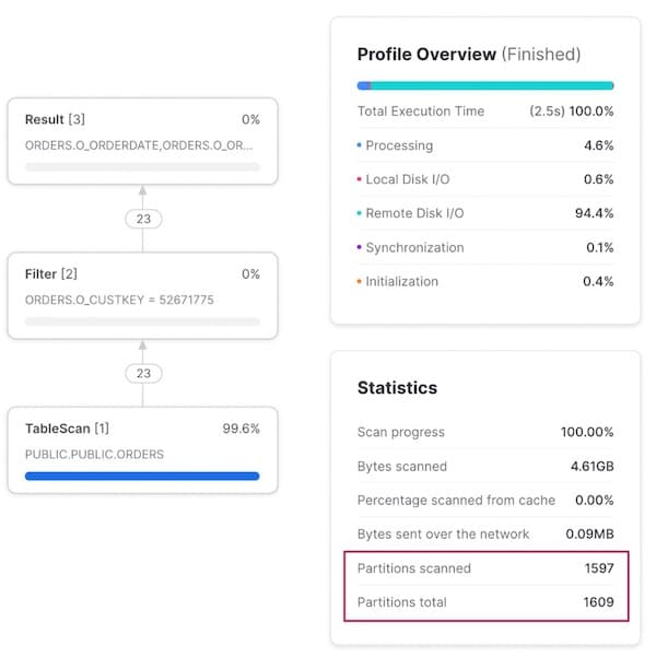
Access Pattern 2: Query for a specific customer

select *
from orders
where o_custkey = 52671775

When we change our query to look up all orders for a particular customer, the query pruning is ineffective with 99% of all micro-partitions being scanned.

Access Pattern 3: Query for a specific order

select *
from orders
where o_orderkey = 5019980134

For our orders based lookup, the third column of our cluster key, we see no pruning whatsoever with all micro-partitions being scanned in order to find our 1 record.

Understanding the degraded performance of multi-column cluster keys

As demonstrated above, the query pruning performance degrades significantly for predicates (filters) on the second and third columns.

To understand why this is the case, it’s important to understand how Snowflake’s clustering works for multi-column cluster keys. The simplest mental model for this is thinking about how you’d organize the data in “boxes of boxes”. Snowflake first groups the data by o_orderdate. Next, within each “date” box, it divides the data by o_custkey. In each of those boxes, it then divides the data by o_orderkey.

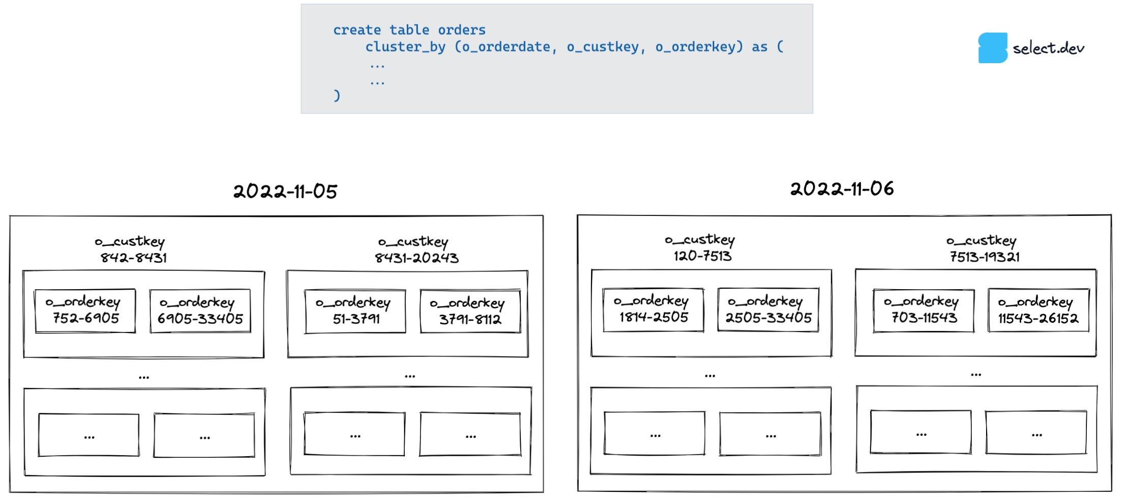
Snowflake’s query pruning works by checking the min/max metadata for the column in each micro-partition. When we query by date, each date has its own dedicated box so we can quickly discard (prune) irrelevant boxes. When we query by customer or order key, we have to check each top-level date box because the min/max value for these columns is a very wide range (a wide range of customers place orders on each day and the order keys are random IDs, not ascending with the order date), so it's not possible to rule out any boxes.

Creating multiple copies of the same table with different cluster keys

As an alternative approach, we could create and maintain a separate table for each cluster key:

create table orders_clustered_by_date cluster by (o_orderdate) as (
  select
    o_orderdate,
    o_orderkey,
    o_custkey,
    o_clerk
  from snowflake_sample_data.tpch_sf1000.orders
)

create table orders_clustered_by_customer cluster by (o_custkey) as (
  select
    o_orderdate,
    o_orderkey,
    o_custkey,
    o_clerk
  from snowflake_sample_data.tpch_sf1000.orders
)

create table orders_clustered_by_order cluster by (o_orderkey) as (
  select
    o_orderdate,
    o_orderkey,
    o_custkey,
    o_clerk
  from snowflake_sample_data.tpch_sf1000.orders
)

This approach has clear downsides. Users now have to keep track of the three different tables and remember which query scenario they should use each table. Not practical for a table that is widely used. You would also be responsible for maintaining the three separate copies of this table in your ETL/ELT pipelines.

Perhaps there’s a better way?

Using clustered, materialized views to leverage Snowflake's powerful automatic pruning optimization feature

What are materialized views?

A materialized view is a pre-computed data set derived from a query specification and stored for later use ². We’ll discuss their use cases in a future post, but for now you can read Snowflake docs which cover them in great detail. When you create a materialized view, like the one below, Snowflake automatically maintains this derived dataset on your behalf. When data is added or modified in the base table (orders), Snowflake automatically updates the materialized view.

create materialized view orders_aggregated_by_date as (
    select
        o_orderdate,
        count(*) as cnt
    from orders
    group by 1
)

Now, if anyone ever runs this query against the base table:

select
    o_orderdate,
    count(*) as cnt
from orders
group by 1

Snowflake will automatically scan the pre-computed materialized view instead of re-computing the entire dataset.

Creating automatically clustered materialized views

Materialized views support automatic clustering. Using this, we can create two new materialized views that separately cluster our orders table by o_custkey and o_orderkey for optimal performance:

-- these will take some time to execute, since the entire dataset is
-- being materialized (created) for the first time
create materialized view orders_clustered_by_customer cluster by(o_custkey) as (
  select
    o_orderdate,
    o_orderkey,
    o_custkey,
    o_clerk
  from orders
)
;

create materialized view orders_clustered_by_order cluster by(o_orderkey) as (
  select
    o_orderdate,
    o_orderkey,
    o_custkey,
    o_clerk
  from orders
)
;

Technically, we could create a third materialized view that is clustered by o_orderdate. Instead, we’ll take the more cost effective approach of leveraging manual sorting on our base orders table:

create table orders as (
  select
    o_orderdate,
    o_orderkey,
    o_custkey,
    o_clerk
  from snowflake_sample_data.tpch_sf1000.orders
  -- sort and therefore cluster the table by o_orderdate
  order by o_orderdate
)

Re-testing our three access patterns

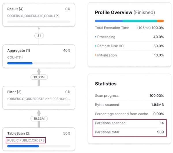
Access Pattern 1: Query by date

select
    o_orderdate,
    count(*) as cnt
from orders
where
    o_orderdate between date'1993-03-01' and date'1993-03-31'
group by 1

When running a query with a filter on o_orderdate, our original base orders tables is used since it is naturally clustered by this column.

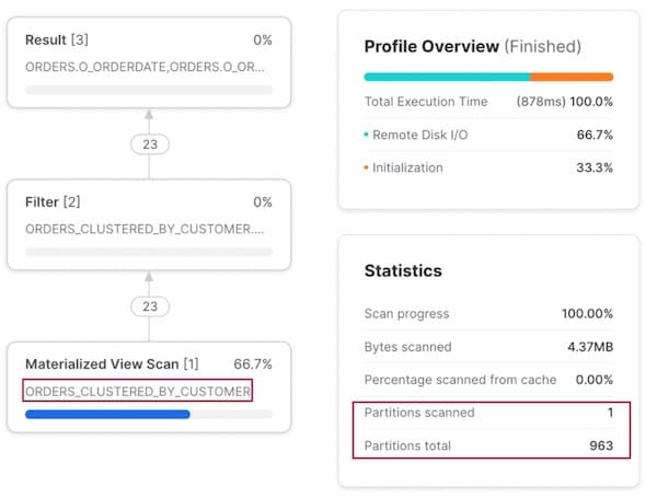
Access Pattern 2: Query by customer

select *
from orders
where
    o_custkey=52671775

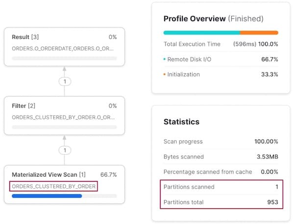
When we instead filter by o_custkey, the Snowflake optimizer recognizes that there is a materialized view clustered by this column, and intelligently instructs the query execution plan to read from the materialized view.

Access Pattern 3: Query by order

select *
from orders
where
    o_orderkey = 5019980134

Filtering on o_orderkey has similar behaviour, with Snowflake “re-routing” the query execution to scan our other materialized view instead of the base orders table.

Clustered materialized view cost considerations

The main downside of using materialized views is the added costs of maintaining the separate materialized views. There are three components to consider:

1. Storage costs associated with the new datasets
2. Charges for the managed refreshes of each materialized view. In order to prevent materialized views from becoming out-of-date, Snowflake performs automatic background maintenance of materialized views. When a base table changes, all materialized views defined on the table are updated by a background service that uses compute resources provided by Snowflake.
3. Charges for automatic clustering on each materialized view. If a materialized view is clustered differently from the base table, the number of micro-partitions changed in the materialized view might be substantially larger than the number of micro-partitions changed in the base table.

We’ll provide more guidance on this in a future post, but for now we recommend monitoring the maintenance costs ³ and automatic clustering costs ⁴ associated with your materialized views. Your can estimate your storage costs upfront based on the table size and your storage costs ⁵.

Materialized view on a clustered table

Each update to your base table triggers a refresh of all associated materialized views. So what happens if both your base table and the materialized view are clustered on different columns?

1. New data gets added to the base table
2. A refresh of the materialized view is triggered
3. Snowflake’s automatic clustering service updates the base table to improve its clustering
4. Automatic clustering also may kick in for the materialized view updated in step 2
5. Once step 3 is completed, that may re-trigger steps 2 and 4 for the materialized view

Materialized views and DML operations

It’s important to note that you’ll only see the performance benefits from materialized views on select style queries. DML operations like updates and deletes won’t benefit. For example, if you run:

update orders
set o_clerk='new clerk'
where o_orderkey=5019980134

The query will do a full table scan on the base orders table and not use the materialized view.

Summary

In this post we showed how materialized views can be leveraged to create multiple versions of a table with different clusters keys. This practice can help significantly improve query performance due to better pruning and even lower the virtual warehouse costs associated with those queries. As with anything in Snowflake, these benefits must be carefully considered against their underlying costs.

In future posts, we’ll explore important topics like how to determine the optimal cluster keys for your table, estimating the costs of automatic clustering for a large table, and how to monitor clustering health and implement more cost effective automatic clustering. We’ll also dive deeper into defining multiple cluster keys on a single table and when it makes sense to do so.

As always, don’t hesitate to reach out via Twitter or email where we'd be happy to answer questions or discuss these topics in more detail. If you want to get notified when we release a new post, be sure to sign up for our Snowflake newsletter at the bottom of this page.

Notes

¹ Notice how we order the clustering keys from lowest to highest cardinality? From the Snowflake documentation on multi-column cluster keys:

If you are defining a multi-column clustering key for a table, the order in which the columns are specified in the CLUSTER BY clause is important. As a general rule, Snowflake recommends ordering the columns from lowest cardinality to highest cardinality. Putting a higher cardinality column before a lower cardinality column will generally reduce the effectiveness of clustering on the latter column.

A column’s cardinality is simply the number of distinct values. You can find this out by running a query:

select
    count(*), -- 1,500,000,000
    count(distinct o_orderdate), -- 2,406
    count(distinct o_orderkey), -- 1,500,000,000
    count(distinct o_custkey) -- 99,999,998
from public.orders

So as a result, we cluster by (o_orderdate, o_custkey, o_orderkey. ↩

² You can only use materialized views if you are on the enterprise (or above) edition of Snowflake. ↩

³ You can monitor the cost of your materialized view refreshes using the following query:

select
    date_trunc(day, start_time) as date,
    table_name as materialized_view_name,
    sum(credits_used) as num_credits_used
from snowflake.account_usage.materialized_view_refresh_history
group by 1,2
order by 1,2

⁴ You can monitor the cost of automatic clustering on your materialized view using the following query:

select
    date_trunc(day, automatic_clustering_history.start_time) as date,
    automatic_clustering_history.database_name || '.' || automatic_clustering_history.schema_name || '.' || automatic_clustering_history.table_name as materialized_view_name,
    sum(credits_used) as num_credits_used
from snowflake.account_usage.automatic_clustering_history
inner join snowflake.account_usage.tables
    on automatic_clustering_history.table_id=tables.table_id
    and tables.table_type='MATERIALIZED VIEW'
group by 1,2
order by 1,2

⁵ Most customers on AWS pay $23/TB/month. So if your base table is 10TB, then each additional materialized view will cost $2,760 / year (10*23*12). ↩