
Snowflake vs Databricks Showdown
Jeff SkoldbergFriday, April 10, 2026
Databricks vs Snowflake. It’s a never ending debate with passionate participants on each side. Years ago these platforms served different audiences, Snowflake for the Analyst and traditional BI team and Databricks for the ML and Data Scientist. Today the feature sets of these platforms is getting much closer to parity with both platforms serving almost all audiences. But that hasn’t stopped the debate. “Snowflake is expensive” or “Databricks is slow”, or [insert random put down] - these stabs are so common on LinkedIn / Reddit, either from enthusiastic fans or from employees of one of the companies.
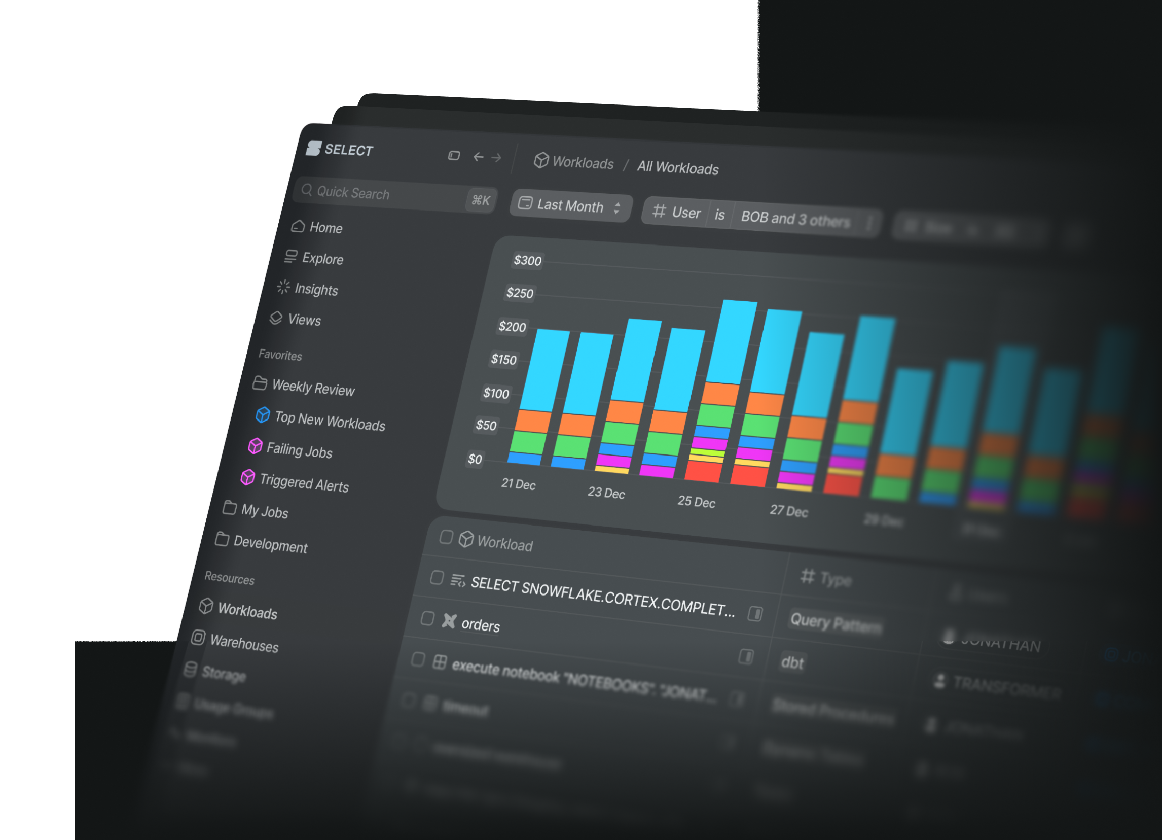
At SELECT, we wanted to run a benchmark that is non-biased, repeatable, and practical. We wanted this to be software driven so that running a Python job would execute the queries and record the results. We wanted this to be designed so new platforms can easily get added to the benchmark. And finally, we wanted a nice visualization on top. We put a lot of effort (maybe an unreasonable amount of effort?) into bringing you this non-biased comparison.
One big caveat before we begin: Benchmarks just tell you how fast the benchmark ran. It doesn’t simulate production workloads and doesn’t predict what will happen on your data with your SQL. While we can draw some conclusions based on this data, definitely experiment using your data and design patterns!
The setup
The Data
Our benchmark uses the TCP-H 1000 Scale Factor. This data set has about 6 billion rows on the largest table. Snowflake and Databricks both have TPC-H data, but they don’t have overlapping sizes or the exact same large data sets. In order to do an apples to apples comparison, you need to ETL the data from Snowflake to Databricks. The easiest way would be to use a tool designed for this like Estuary, or you can do this on your own.
Databricks comes with:
- tpcds_sf1 and sf1000
- tpch with 30 million rows. This is about 1/2 the size of Snowflakes 10 scale factor, which has 60 million rows.
Snowflake comes with:
- tpcds_sf10 and 100
- tpch at scale factors 1, 10, 100, and 1000
No surprise, the platforms made it hard to compare performance by not providing similar sample data. 🤨
Scenarios
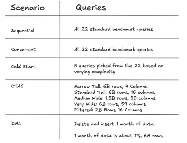
We used these existing standard queries under 3 scenarios:
- Run all 22 queries sequentially. In this scenario, only query 1 is a cold start and each subsequent query can benefit from the warehouse cache of the queries that came before it.
- Run all 22 queries concurrently. In this scenario we’re testing the data platform’s ability to run multiple queries at once and to see of any horizontal scaling is observed.
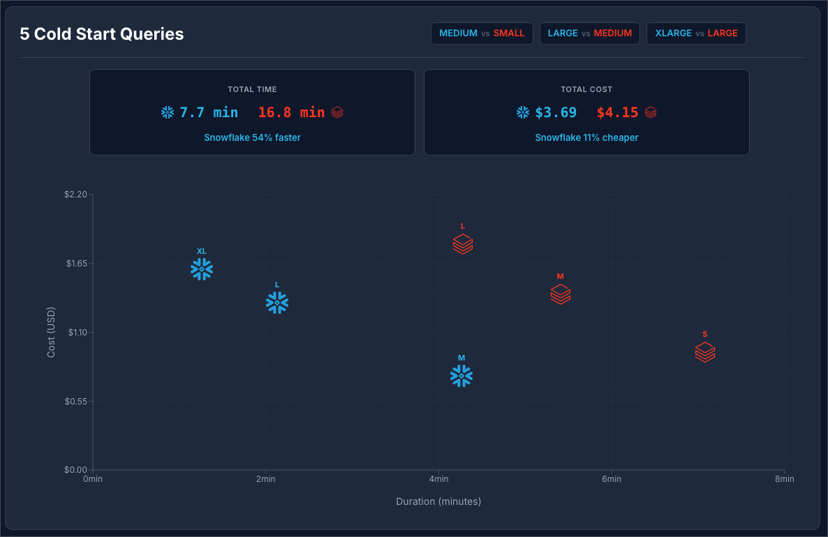
- 5 cold start queries. We ran a small selection of the queries, varying complexity and style, to see how the platforms compared when run on cold warehouse.
CTAS Workloads: Since the standard benchmark queries produce a small-ish result and most are highly aggregated, they were not a good indication of a real CTAS workload because the write payload would be too small to stress-test write throughput. To test write-intensive operations, we created 5 variants that materialize large result sets with different data shapes, ranging from narrow tables with billions of rows to very wide denormalized tables, allowing us to compare write performance on different table shapes and query complexity.
DML Workloads: Here we are deleting 1 month of data from the table and re-inserting it. 1 month represents about 1% of the data or 6M rows. This will be a test of both query pruning efficiency (targeting the 1 month), as well as DML efficiency.
Warehouses
Each run and scenario has a new warehouse auto-generated at the beginning of that run + scenario, then the warehouse is destroyed immediately when the work is done. This allows us to look at the total cost of a warehouse in isolation and eliminate idle time from the picture.
A Databricks Severless SQL Warehouse is roughly equivalent to a Snowflake Warehouse that is one size larger. Example, a Small in Databricks is roughly equivalent to a Medium in Snowflake. We ran the 4 scenarios above on these warehouse combinations.
- Snowflake Medium vs Databricks Small
- Snowflake Large vs Databricks Medium
- Snowflake XL vs Databricks Large
This comparison of sizes is corroborated by Snowflake and Databricks documentation, where the Databricks Worker Count is assumed to be equal to the Snowflake Credits.
Cost attribution
We wanted the cost attribution to be as perfect as possible. To achieve this, isolated warehouses are used as described above. We use the actual billing data (in credits or DBUs) for the life of that warehouse. In the end we use a flexible cost calculator to apply various cost per credit or cost per DBU to the results to simulate different platform tiers. By taking this approach we eliminate all complexity of cost attribution for concurrent running queries or minimum billing increments, etc. We just look at the total cost for the scenario.
When we show cost for individual queries instead of entire runs, the cost is attributed to that query based on the proportion of its run time. Basically the total cost for the run (or the lifetime of that warehouse) is spread across the queries so the numbers add up.
Cost Comparison
The Databricks Standard Tier is being retired (or likely was retired in Oct 2025). Therefore if we are to compare the lowest List Price for each platform the comparison would be Snowflake Standard at $2 / credit vs Databricks Enterprise at $0.70 / DBU. We feel this is a fair comparison since the Snowflake Standard tier is a full-fledged version of Snowflake, with the main missing feature being time travel. However, we understand that many readers will want to compare Enterprise vs Enterprise. So, we will show both: Databricks at $0.70 / DBU vs Snowflake at $2 / credit and at $3 / credit.
Run History and Analysis
Query IDs and run stats are immediately logged to a local duckdb. The data is stored at the query ID grain (plus run ID, Warehouse, scenario). Reporting views roll up the data so we can draw conclusions across entire runs.
Queries
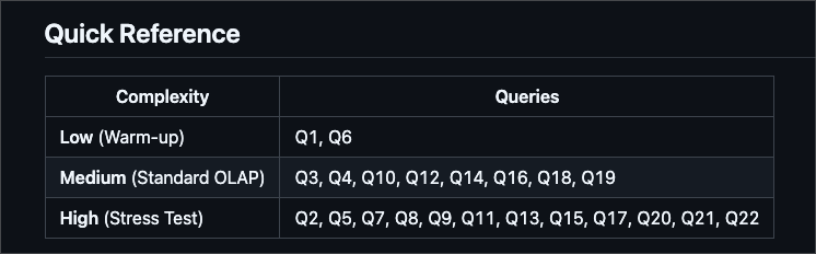
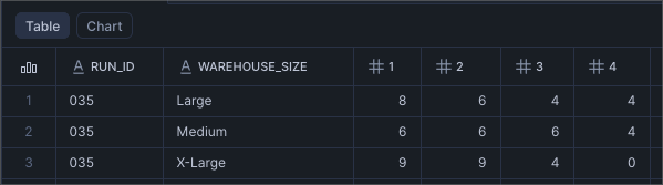
The benchmarking queries can be found here. (Although the SQL looks like it is hard-coded to the 100x scale factor data, the table name is dynamically replaced at run time with the scale factor in your config file. All tests were run on 1000x scale factor). We have organized the 22 queries into categories based on complexity and number of joins. The detailed category breakdown can be found here, but this screenshot provides a brief summary.
Scenario 1: 22 Sequential Queries
Goal and Setup
Goal: Running queries sequentially mimics what you may experience sitting at your desk and running queries on these data platforms. This is what end users will experience when they run a select query. This measurement gives us the ability to compare query by query, warehouse by warehouse in a similar way to most TPC-H benchmarks.
Setup: The setup is dead simple: We run 22 queries, one at a time. In all scenarios the warehouse is created at the beginning of the run and destroyed immediately after the last query finishes. Query results are immediately logged to the duckdb.
In this scenario only query 1 is a true “cold start” and queries 2-22 are considered warm, as the warehouse remains on for the entire run.
Results
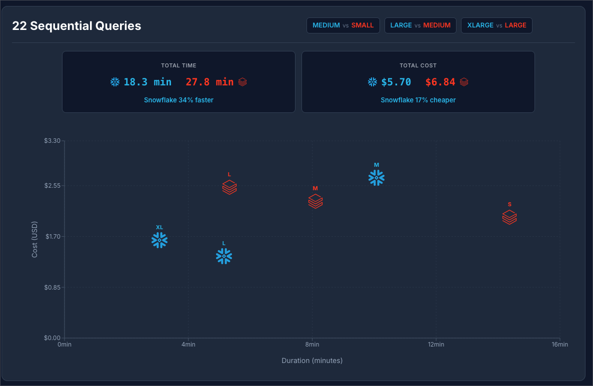
Snowflake at $2 / Credit vs Databricks at $0.70 / DBU:
Snowflake at $3 / Credit vs Databricks at $0.70 / DBU:
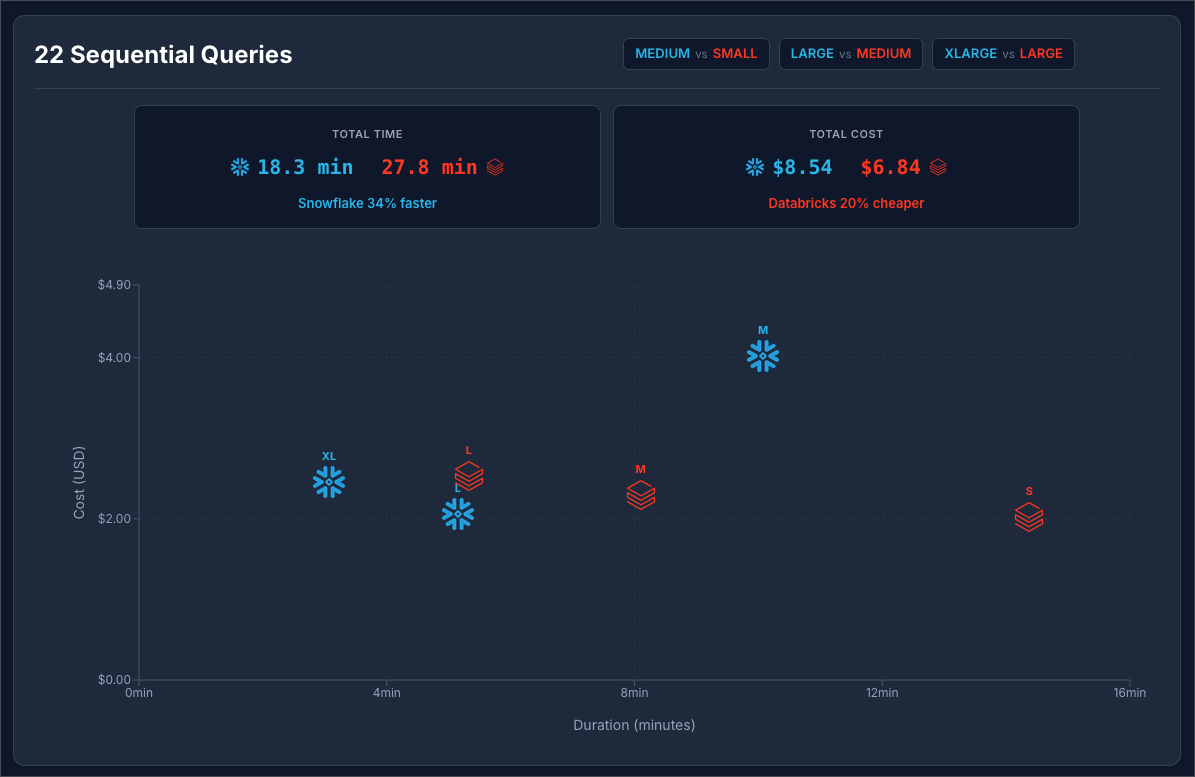
You can see at $2 / Credit Snowflake is 34% faster and 17% cheaper. Moving Snowflake to to $3 / credit makes Databricks 20% cheaper.
Scenario 2: 22 Concurrent Queries
Goal and Setup
Goal: This simulates loading a BI dashboard or running jobs where dozens of queries are fired at once. The goal is to test how each data platform handles concurrency.
Setup: We used Python to fire all 22 queries at once and record the results.
Results
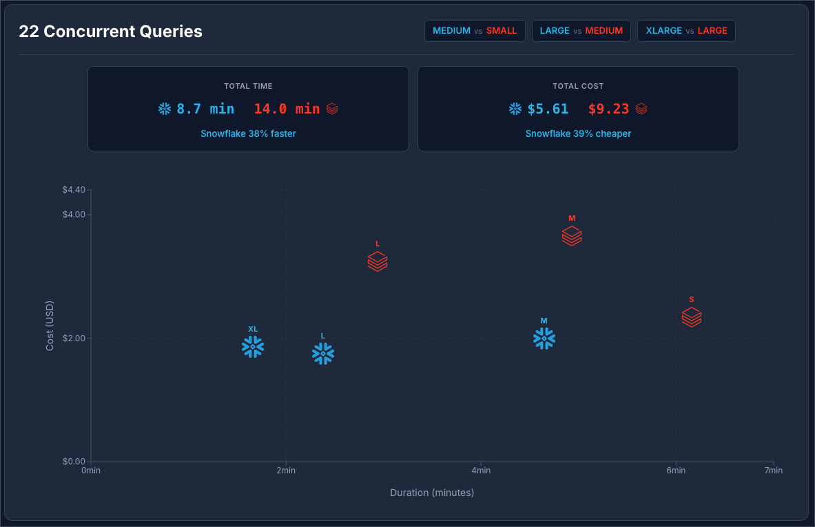
Snowflake at $2 / Credit vs Databricks at $0.70 / DBU:
Snowflake at $3 / Credit vs Databricks at $0.70 / DBU:
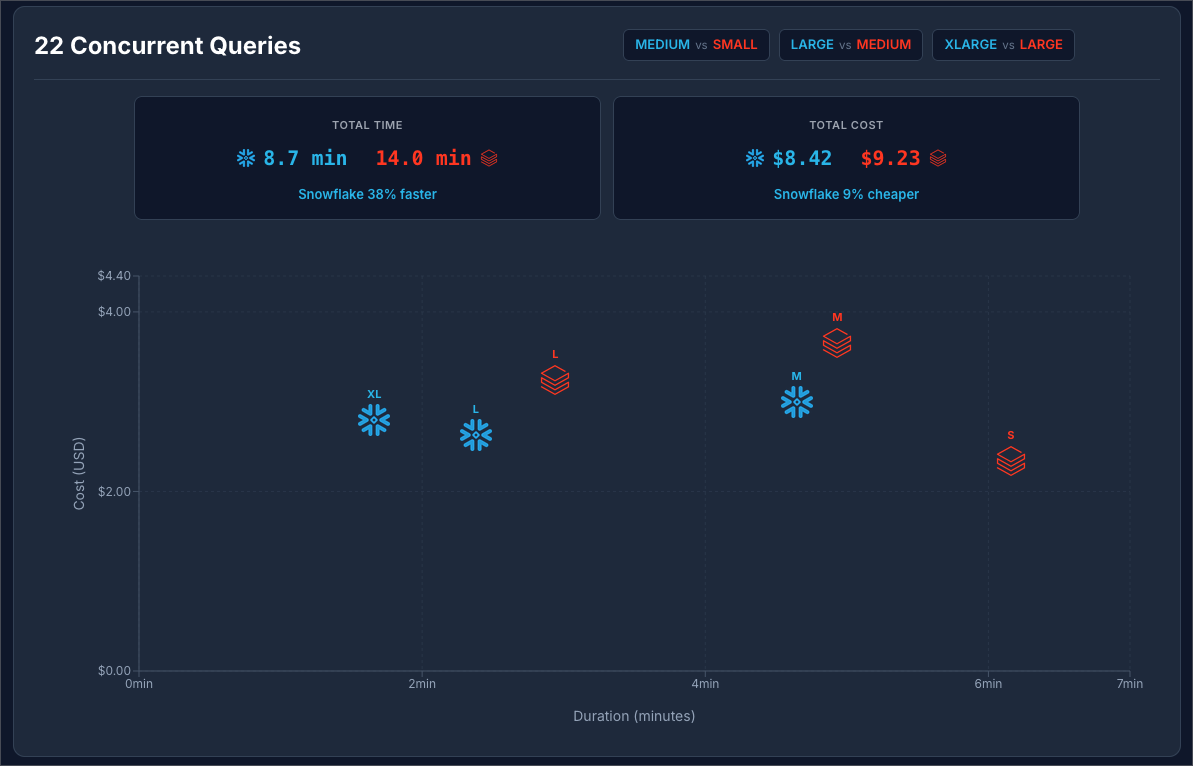
In both scenarios, Snowflake was faster and cheaper! This means for concurrent workloads Snowflake seems to be the winner (in this benchmark scenario).
But now let’s explore how will each platform handled the concurrency. If concurrency is handled perfectly (no queuing or resource competition), the total run time of the concurrent test should be about the same as the longest running query run by itself.
| Platform | Warehouse Size | Longest Isolated Query | Concurrent Wallclock | Ratio |
|---|---|---|---|---|
| Databricks | SMALL | 134.5 sec | 369.5 sec | 2.7x |
| Databricks | MEDIUM | 64.5 sec | 296.0 sec | 4.6x |
| Databricks | LARGE | 32.9 sec | 176.5 sec | 5.4x |
| Snowflake | MEDIUM | 94.7 sec | 278.7 sec | 2.9x |
| Snowflake | LARGE | 45.2 sec | 142.8 sec | 3.2x |
| Snowflake | XLARGE | 20.7 sec | 99.7 sec | 4.8x |
The data above shows that in both platforms there is a penalty for running concurrent queries, (running multiple queries at once makes them all slower or there is queuing), but Snowflake has the better ratio on this comparison.
Running 22 concurrent queries we can see that Snowflake scaled up to 4 clusters for Medium and Large and only used 3 clusters on the XL. This why the XL only cost a few cents more than the Large.
Unfortunately the same data is not available in Databricks. I was not able to find a way to tell how many clusters were utilized.
Scenario 3: Cold Start
Goal and setup
Goals: to measure query run times with no “Warehouse cache” and to see if warehouse startup time impacts the results.
Both platforms leverage “warehouse cache” or “Photon acceleration”, a cache that lives on the VM running the query. When running queries sequentially, query 2 can benefit from some of the cache generated by query 1, etc.
Setup: In order to see how queries performed when no cache was available, we designed a scenario that shuts down the warehouse between each query execution. In this case we decided to not run all 22 queries, this would cause a lot of excess spend.
Warehouse creation time is not counted in the total wall clock time, but warehouse startup time IS counted in the total wall clock time.
The queries
| Query | Category | Complexity | Description |
|---|---|---|---|
| Q1 | Simple Aggregation & Filtering | Low (Warm-up) | Multiple aggregations (SUM, AVG, COUNT) with GROUP BY on 600M row table |
| Q3 | Basic Joins (2-4 tables) | Medium (Standard OLAP) | 3-way join with aggregation and date filtering |
| Q5 | Complex Joins (5+ tables) | High (Stress Test) | 6-way join with revenue calculation and geographic filtering |
| Q10 | Basic Joins (2-4 tables) | Medium (Standard OLAP) | 4-way join with selective filter and high-cardinality GROUP BY |
| Q18 | Subqueries & Semi-Joins | Medium (Standard OLAP) | IN subquery with aggregation filter (HAVING) |
Query Category Complexity Description Q1 Simple Aggregation & Filtering Low (Warm-up) Multiple aggregations (SUM, AVG, COUNT) with GROUP BY on 600M row table Q3 Basic Joins (2-4 tables) Medium (Standard OLAP) 3-way join with aggregation and date filtering Q5 Complex Joins (5+ tables) High (Stress Test) 6-way join with revenue calculation and geographic filtering Q10 Basic Joins (2-4 tables) Medium (Standard OLAP) 4-way join with selective filter and high-cardinality GROUP BY Q18 Subqueries & Semi-Joins Medium (Standard OLAP) IN subquery with aggregation filter (HAVING)
Results
Here we can see that Snowflake was orders of magnitude faster and a bit cheaper.
Looking at the details, we found that Databricks startup time was roughly 7 seconds per start and Snowflake startup time was sub-second in all cases.
Scenario 4: CTAS (Create Table As Select)
Goal and Setup
Goal: The goal is to measure write intensive operations typical of data engineering tasks and dbt projects. The standard TPC-H queries are optimized for analytical reads; they scan large datasets but return small, aggregated results (sums, averages, top-N lists). While this tests query execution and optimization, it doesn't stress-test write performance. We wanted to understand how Snowflake and Databricks compare when writing billions of rows with varying data shapes.
Setup: We created 5 CTAS variants, each designed to test a specific write pattern:
- Narrow Tall (6B rows × 4 columns): A simple projection of the LINEITEM table with just 4 key columns (l_orderkey, l_partkey, l_quantity, l_extendedprice). This tests maximum row throughput with minimal column overhead.
- Standard Tall (6B rows × 16 columns): A full copy of the LINEITEM table (SELECT * FROM LINEITEM). This represents a common pattern of duplicating or archiving large fact tables. (Usually you would use Clone for this, but we’re not benchmarking Clone operations today.)
- Medium Wide (1.5B rows × 30 columns): A join of ORDERS, CUSTOMER, NATION, and REGION tables. This tests combining read and write performance with moderate JOIN complexity and a wider schema, typical of star schema denormalization.
- Very Wide (6B rows × 59 columns): A fully denormalized join across all TPC-H tables (LINEITEM, ORDERS, CUSTOMER, SUPPLIER, PART, PARTSUPP, NATION, REGION). This represents the extreme case of wide, pre-joined tables common in analytics layers.
- Filtered (2B rows × 16 columns): LINEITEM filtered to orders shipped after 1995 (WHERE l_shipdate >= '1995-01-01'). This tests write throughput for partial table copies, which is a common pattern in incremental data pipelines.
Results
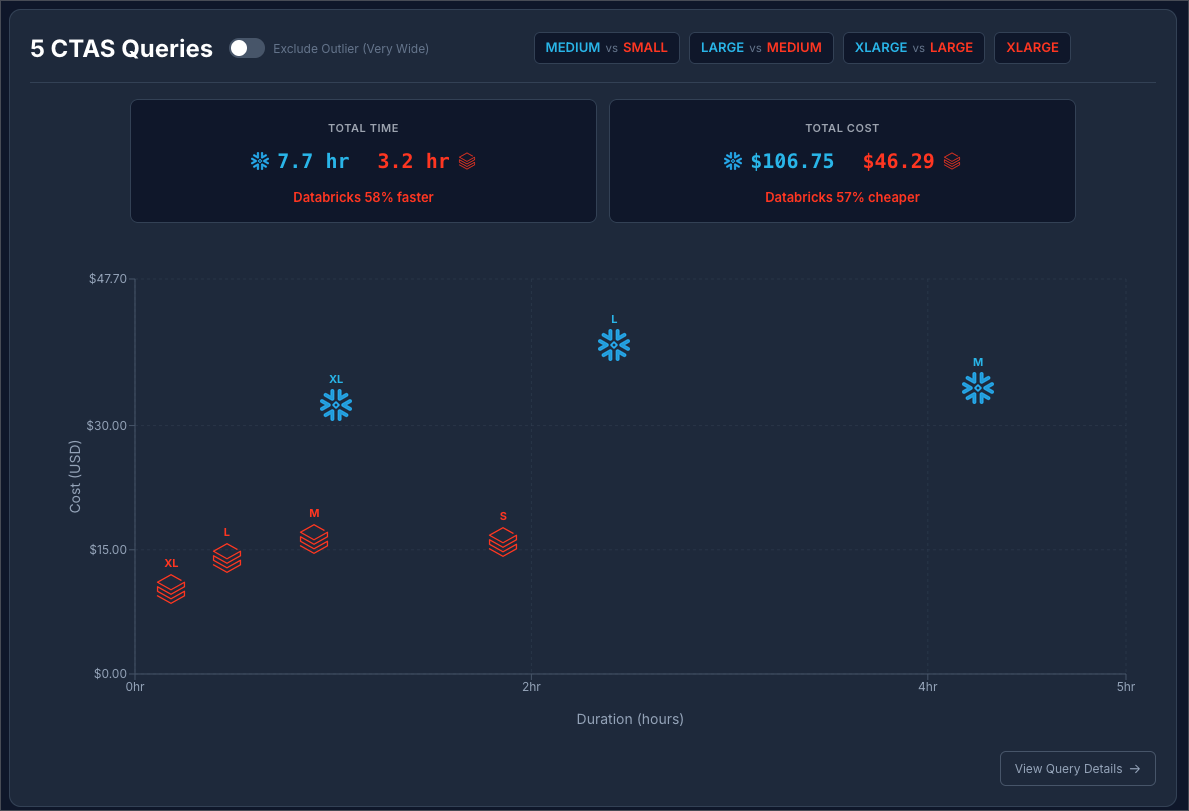
Snowflake at $2 / Credit vs Databricks at $0.70 / DBU:
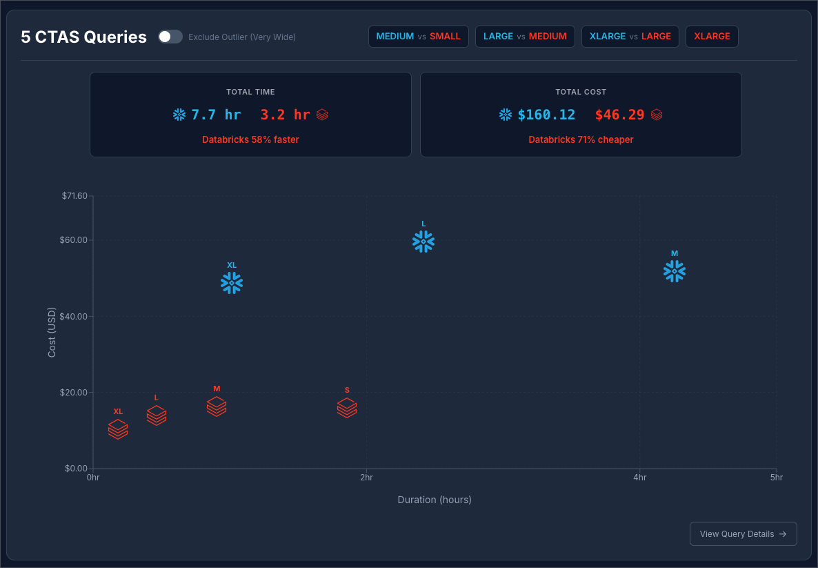
Snowflake at $3 / Credit vs Databricks at $0.70 / DBU:
Snowflake at $2 / Credit vs Databricks at $0.70 / DBU, excluding the “Very Wide” outlier query:
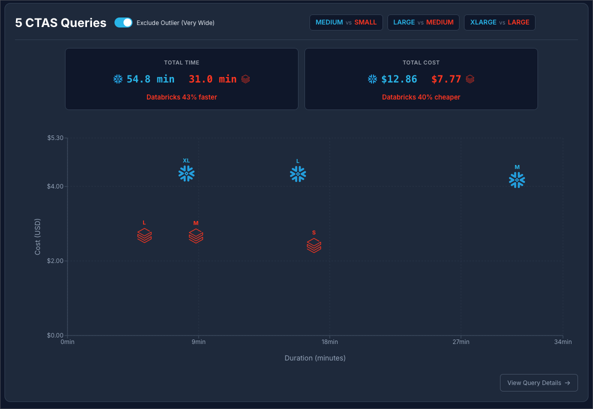
Snowflake at $3 / Credit vs Databricks at $0.70 / DBU, excluding the “Very Wide” outlier query:
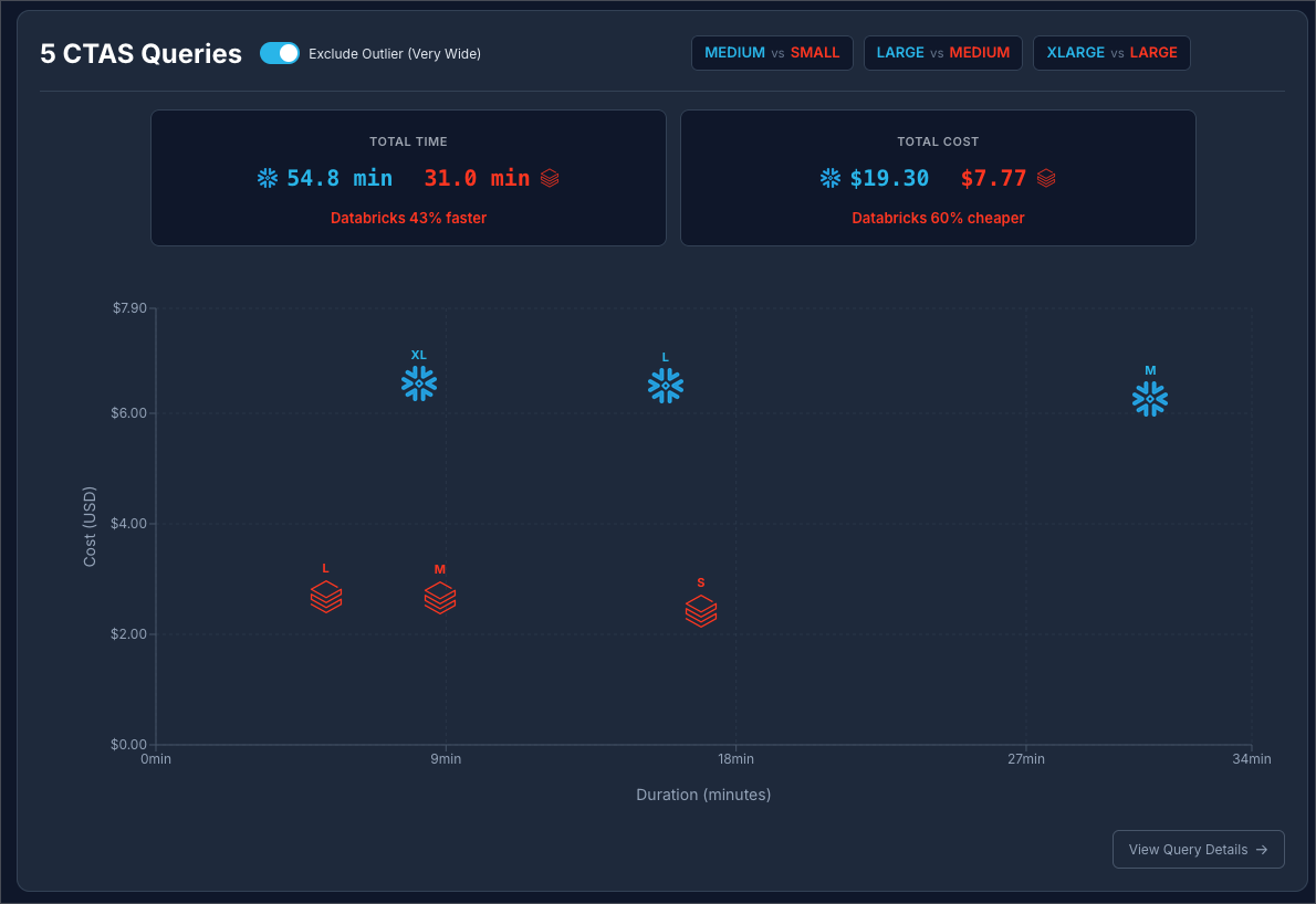
It is safe to say that in this benchmark scenario, Databricks has a strong edge at creating large tables using CTAS.
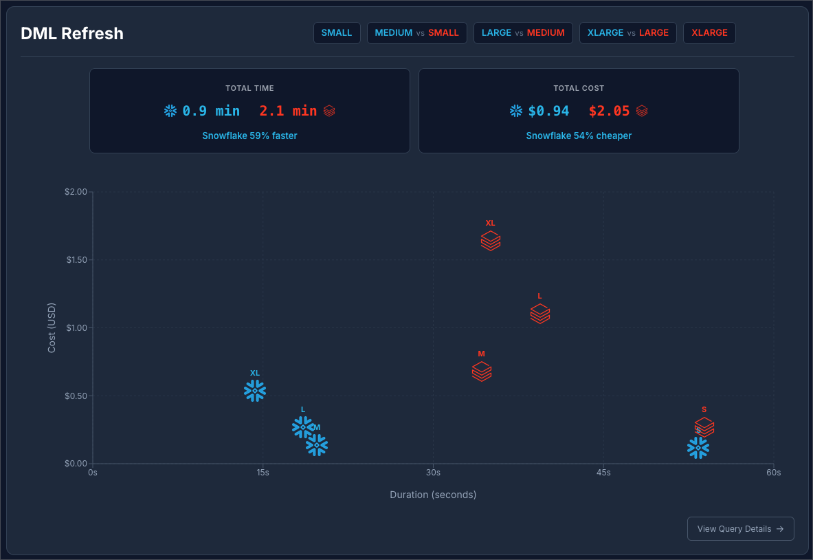
Scenario 5: DML (Data Manipulation Language)
Goal and Setup
Goal: Delete + Insert is a common pattern to update data incrementally. This is the most effective way to transform targeted segments of data on large tables, and therefore an important scenario to test.
Setup: At the beginning of the run, a copy of the source benchmark data is created. This is not counted in the run time or the cost metrics. Once the copy of the data is created, the benchmark process begins. It delete 1 month of data, about 6M rows or about 1% of the total data. Then re-insert the same month from the source. This simulates a real-life ETL scenario where matched records are deleted + inserted. Note, we did not use merge because it is well know that delete + insert outperforms merge.
Results
Snowflake at $2 / Credit vs Databricks at $0.70 / DBU:
Snowflake at $3 / Credit vs Databricks at $0.70 / DBU:
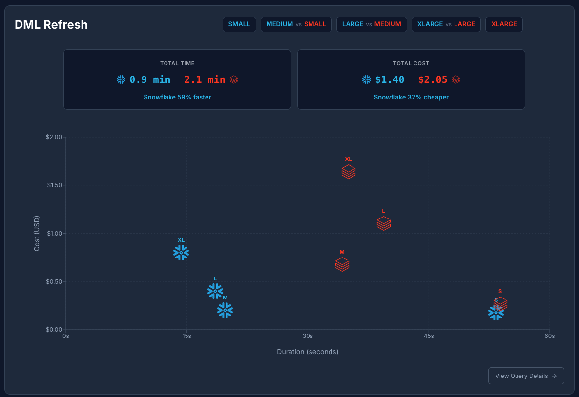
The results are really interesting here. The reason why Snowflake M, L, and XL all process the data in less than 20 seconds is because of excellent query pruning. The 6 billion rows is pruned to be treated like 6 million rows, so it operates on a much smaller data set. The Small Snowflake warehouse takes more than twice as long because it experiences spillage on both the delete and insert steps.
The same thing is happening on Databricks. We see a concentration between 35 and 39 seconds for all of the warehouse sizes. Databricks is effectively reducing the size of the dataset, so M, L, and XL handle it with no problem. But just not quite as fast as Snowflake.
Reproducing this benchmark
If you’d like to run these tests for yourself, it is relatively easy to do so. As mentioned above, the first thing you need to do is ETL the 1000x data set from Snowflake to Databricks. This is the hard part, and the only part we are not providing automation for since there are too many variables at play. Again, I recommend using Estuary for this!
Once the data is available in your Databricks account, you can follow the getting started, here. You just need to have UV and Snowflake CLI installed, set up your .env file by running uv run setup_config.py, then you can start running benchmarks! The readme has plenty examples of how to run individual scenarios, warehouse sizes, or just run the whole thing wide open.
After the benchmark runs, you need to wait 2 hours for the billing data to settle. Then you can run uv run enrich.py to enrich the results with the billing data. When you’re ready to visualize the results, you follow the readme steps to do that as well.
Wrap Up
The results conclusively show that Snowflake Standard Edition is the most cost effective platform for all scenarios except the CTAS scenario where Databricks outperforms Snowflake in terms of both cost and performance. Upgrading to Snowflake Enterprise Edition at $3 / credit makes Databricks cheaper in some scenarios. Again, benchmarks are just benchmarks, so be sure to test on your own data!

Jeff is a Data and Analytics Consultant with 15+ years experience in automating insights and using data to control business processes. From a technology standpoint, he specializes in Snowflake + dbt + Tableau. From a business topic standpoint, he has experience in Public Utility, Clinical Trials, Publishing, CPG, and Manufacturing. Reach out any time, [email protected].
Want to hear about our latest data cloud learnings?Subscribe to get notified.
Get up and running in less than 15 minutes
Connect your Snowflake, Databricks, or BigQuery account and instantly understand your savings potential.